
Past-future Mutual Information Estimation in Sparse Information
Conditions
Yuval Shalev
a
and Irad Ben-Gal
b
Laboratory for AI, Machine Learning, Business & Data Analytics, Department of Industrial Engineering,
Keywords:
Past-future Mutual Information, Context Tree, Transfer Entropy, Time Series Analysis.
Abstract:
We introduce the CT-PFMI, a context tree based algorithm that estimates the past-future mutual information
(PFMI) between different time series. By applying a pruning phase of the context tree algorithm, uninfor-
mative past sequences are removed from PFMI estimation along with their false contributions. In situations
where most of the past data is uninformative, the CT-PFMI shows better estimates to the true PFMI than other
benchmark methods as demonstrated in a simulated study. By implementing CT-PFMI on real stock prices
data we also demonstrate how the algorithm provides useful insights when analyzing the interactions between
financial time series.
1 INTRODUCTION
Accurate estimation of the mutual information be-
tween the past of one time series and the future of
another is an important task in time series analysis.
For instance, the transfer entropy (Schreiber, 2000),
that measures the conditional past-future mutual in-
formation (PFMI) between the past of one or more
time series and an output time series that are condi-
tioned on the past of the output time series, has been
widely explored in the past two decades in various do-
mains such as neural-science and economics (Bosso-
maier et al., 2016). However, a difficulty arises when
PFMI needs to be estimated from data observations.
The number of possible sequences that potentially
contributes to the mutual information increases expo-
nentially with the number of time lags. When most
realized past sequences are uninformative about the
future, a condition we call sparse PFMI, large num-
ber of false contributors could lead to overestimation
of PFMI, hence associating predictive power to unin-
formative sequences.
The methods that are used to estimate PFMI, usu-
ally in the context of transfer entropy estimation,
are based on commonly used MI estimation meth-
ods ranging from naive binning (also called the Plug-
in method) to bias and variance corrections such as
the nearest neighbors method (Montalto et al., 2014;
a
https://orcid.org/0000-0003-2125-9735
b
https://orcid.org/0000-0003-2411-5518
Runge et al., 2012). When applied to time series,
these methods resolve the time dimensionality prob-
lem by removing uninformative time lags entirely.
Nevertheless, to the best of our knowledge, none of
these methods apply estimation correction at a real-
ization level, which has a greater potential for dimen-
sionality reduction and can provide an insightful per-
spective on the nature of the underlying interactions.
We provide such a solution by estimating the
PFMI using an expansion of the context tree (CT) al-
gorithm which is called the input/output context tree
(I/O CT) algorithm (Ben-Gal et al., 2005; Brice and
Jiang, 2009). This algorithm parses the input time
series into a tree of contexts (sequences), where in
each node, the conditional probability of the out-
put given the context is assigned. Next, only nodes
with conditional probabilities that are significantly
different from those of their parent nodes (often mea-
sured by the Kullback-Liebler divergence) are kept,
and the others are pruned. This algorithm, as well
as other algorithms from the Variable Order Markov
Models family, were proposed to overcome overfit-
ting in learning tasks such as classification and pre-
diction (Ben-Gal et al., 2005; Begleiter et al., 2004;
Shmilovici and Ben-Gal, 2012; Yang et al., 2014). Es-
timating the information between a time series’ past
and future was usually not one of the tasks these al-
gorithms were used for. We show how to estimate
PFMI between time series as the sum of the Kullback-
Leibler divergence (Kullback and Leibler, 1951) be-
Shalev, Y. and Ben-Gal, I.
Past-future Mutual Information Estimation in Sparse Information Conditions.
DOI: 10.5220/0008069300650071
In Proceedings of the 11th International Joint Conference on Knowledge Discovery, Knowledge Engineering and Knowledge Management (IC3K 2019), pages 65-71
ISBN: 978-989-758-382-7
Copyright
c
2019 by SCITEPRESS – Science and Technology Publications, Lda. All rights reserved
65

tween the root node and the leaves of I/O CT. The
proposed procedure is implemented by a proposed
context tree past-future mutual information algorithm
(CT-PFMI): First, a full I/O CT is built. Second, the
PFMI is calculated for descending values of the prun-
ing constant c, a positive parameter which defines the
number of pruned sequences(Ben-Gal et al., 2003).
Third, by identifying the threshold at which redun-
dant information is removed, a value of c is chosen to
obtain an estimate for the "filtered" PFMI as well as
most of the informative sequences.
In the results section it is shown that in simulated
sparse PFMI condition, the CT-PFMI estimates the
PFMI more accurately than benchmark methods. The
proposed CT-PFMI is also implemented on real time
series of stock prices returns, that due to market effi-
ciency, follow the sparse PFMI condition (Shmilovici
and Ben-Gal, 2012). The outcome of the CT-PFMI
algorithm can also be exploited to gain important in-
sights by performing a higher-resolution analysis of
the PFMI contributors as demonstrated by real time
series data.
To conclude, the first contribution of this paper is
to demonstrate the extraction of PFMI from an I/O CT
constructed from input and output time series. The
second contribution is the introduction of a novel al-
gorithm, called the CT-PFMI. This algorithm, is used
for PFMI estimation, while offering a new method of
identifying the value of the pruning constant that gov-
erns the compression rate. The third contribution is
showing how the CT-PFMI algorithm can be used for
in-depth analysis of interaction’s insights in the data.
2 RELATED WORK
In the previous section we mentioned the works on
transfer entropy (Schreiber, 2000; Bossomaier et al.,
2016) as an important source for discussion on esti-
mating the information flow between the past and the
future of time series.
Researchers such as (Runge et al., 2012; Montalto
et al., 2014) used standard methods of MI estimation,
such as binning (Cover and Thomas, 2012) or nearest-
neighbours (Kraskov et al., 2004), to estimate TE. Ac-
cording to those methods, when a specific time lag is
found to be informative in some specific realizations,
all its realizations, including the uninformative ones,
are included in the estimation. In sequential data,
where the number of different realizations is poten-
tially large, this drawback can be crucial by adding
many uninformative sequences to the estimation af-
fecting both the TE accuracy as well as the extracted
insights from the data.
To overcome this challenge, we utilize the CT
algorithm, a member of the family of Variable Or-
der Markov Models that were originally constructed
for compression of a single time series, and found
it to be well-suited to the prediction task of discrete
time series (Weinberger et al., 1995; Begleiter et al.,
2004; Shmilovici and Ben-Gal, 2012). Variable Or-
der Markov Models and their usage have been exten-
sively explored (Begleiter et al., 2004; Shmilovici and
Ben-Gal, 2012; Yang et al., 2014; Slonim et al., 2003;
Largeron-Leténo, 2003; Society et al., 2014; Chim
and Deng, 2007; Ben-Gal et al., 2003; Begleiter et al.,
2013; Ben-Gal et al., 2005; Kusters and Ignatenko,
2015). Two works were found that incorporated Vari-
able Order models and information or entropy (Schür-
mann and Grassberger, 1996; Slonim et al., 2003), yet
none of them used these models for PFMI estimation.
Ben-Gal et al (Ben-Gal et al., 2005) and later
Brice et al (Brice and Jiang, 2009) proposed an in-
put/output formulation of the context tree algorithm
(I/O CT), where the branches of the context tree be-
long to one time series and the leaves belong to an-
other time series. In this way, the researchers could
incorporate data from different time series for learn-
ing tasks, such as structure learning and anomaly de-
tection within the CT framework.
Let us also note that the CT-PFMI algorithm is
scalable using methods presented in (Satish et al.,
2014; Kaniwa et al., 2017; Tiwari and Arya, 2018;
Satish et al., 2014; Tiwari and Arya, 2018).
3 PRELIMINARIES AND
MATHEMATICAL
BACKGROUND
Henceforth, unless stated otherwise, random vari-
ables are represented by capital letters, while their
realizations are denoted by lower-case letters; multi-
dimensional variables and arrays are denoted by bold
letters.
Mutual Information(Cover and Thomas, 2012):
Given two discrete random variables X and Y, the
Mutual Information between them is defined as
IpX ;Y q “
ÿ
xPX
ÿ
yPY
Ppx, yqlog
Ppx, yq
PpxqPpyq
. (1)
IpX ;Y q is a positive symmetrical measure. The
Kullback-Liebler divergence (D
KL
) between arbitrary
probability functions Qp¨q and Pp¨q is given by
KDIR 2019 - 11th International Conference on Knowledge Discovery and Information Retrieval
66

D
KL
pQpX, Y q k PpX, Y qq “
ÿ
xPX
ÿ
yPY
Qpx, yq log
Qpx, yq
Ppx, yq
.
(2)
Following Eq.(2), the IpX ;Y q can be written as
IpX ;Y q “ xD
KL
pPpY |X q k PpY qqy
PpXq
, (3)
where x¨y
Pp¨q
is the expectation with respect to the
subscript distribution.
The Past-future Mutual Information: To explain
PFMI, we use the notation in (Bialek et al., 2001;
Still, 2014) whom introduce a similar measure to
PFMI called the predictive information (PI), that is
the mutual information between two random vectors,
one representing the past τ
p
time lags,
ÐÝ
X
τ
p
and an-
other representing time series values from the future
τ
f
time lags,
ÝÑ
Y
τ
f
. Following Eq.(3), the PI can be
defined by using D
KL
PIp
ÐÝ
X
τ
p
;
ÝÑ
Y
τ
f
q “
xD
KL
pPp
ÝÑ
X
τ
f
|
ÐÝ
X
τ
p
q k Pp
ÝÑ
Y
τ
f
qqy
Pp
ÐÝ
X
τ
p
q
.
(4)
and,
PIp
ÐÝ
X
τ
p
;
ÝÑ
Y
τ
f “1
q “ PFMIp
ÐÝ
X
τ
p
;
ÝÑ
Y q. (5)
Context Tree (CT) Algorithm (Weinberger et al.,
1995; Ben-Gal et al., 2003): Given a sequence of
length N, x
N
, generated from a tree source X , the CT
algorithm finds a finite set S of size |S | of contexts
S px
N
q. S satisfies the requirement that the conditional
probability to obtain a symbol given the whole se-
quence preceding that symbol is close enough to the
Table 1: Optimal contexts of the I/O CT of Deutsche Bank
(input) to HSBC (output) as obtained with the CT-PFMI
algorithm and the pruning constant tuning algorithms (see
Section 5). The returns are discretized to "1" for positive
return, "0" for zero return and "-1" for negative return with
respect to the previous minute.
Optimal Context
Context
Probability Conditional probability
root - (0.42, 0.16, 0.42)
("-1") 0.369 (0.45, 0.15, 0.40)
("0") 0.111 (0.40, 0.20, 0.40)
("1") 0.370 (0.40, 0.15, 0.45)
("-1", "0") 0.057 (0.43, 0.20, 0.37)
("1", "0") 0.058 (0.37, 0.20, 0.43)
("0", "0") 0.011 (0.37, 0.27, 0.36)
("0", "0", "1") 0.011 (0.36, 0.25, 0.39)
("0", "0", "0", "-1") 0.003 (0.35, 0.30, 0.35)
("0", "0", "0", "1") 0.003 (0.33, 0.30, 0.37)
("0", "0", "0", "0") 0.002 (0.32, 0.33, 0.35)
("0", "0", "0", "0", "0") 0.005 (0.06, 0.87, 0.07)
conditional probability of obtaining the symbol given
a context, i.e.,
Ppx|x
N
q – Ppx|S px
N
qq. (6)
Given Eq.(6), when |S | sequences are informative, the
number of conditional probability parameters that are
required to describe x
N
equals |S |(d-1), where d is the
alphabet size of X.
To obtain S , the learning algorithm constructs a
context tree where each node holds a set of ordered
counters that represent the distribution of symbols
that follow that context, which is defined by the path
to that node (Ben-Gal et al., 2003). At the next step,
a pruning procedure is performed to leave only those
contexts in S (called optimal contexts (Ben-Gal et al.,
2003)) - with corresponding nodes in the tree that rep-
resent the conditional distribution of the output vari-
able conditioned on the context which is different
from the distributions of the output variable condi-
tioned only on part of the context (represented by the
path from the tree root to the parent node). Table 1
shows all the optimal contexts and their correspond-
ing conditional probabilities in a I/O context tree ob-
tained in stock returns data that will be discussed in
the result section. Fig. 1 shows in a context tree for-
mation some of the optimal contexts obtained in this
table.
Descriptions of the main principles of the CT Al-
gorithm, including how to obtain S and a numerical
example appear in (Ben-Gal et al., 2003).
The I/O CT (Ben-Gal et al., 2005; Brice and Jiang,
2009) algorithm is a generalization of the CT algo-
rithm where the tree’s contexts are from the input se-
quence and the leaves represent counters of the output
sequence, in contrast to Eq.(6), where the input and
the output are from the same time series
Ppy|x
N
q – Ppy|S px
N
qq. (7)
4 THE CONTEXT TREE
PAST-FUTURE MUTUAL
INFORMATION ALGORITHM
Let t
ÐÝ
x ;
˜
ÐÝ
x u P
ÐÝ
x
τ
p
represent the informative and un-
informative contexts respectively from the input time
series,
ÝÑ
y represents the symbols from the output
time series and
{
PFMIp
ÐÝ
x
τ
p
;
ÝÑ
y q represent the esti-
mated PFMI. We define the uninformative sequences
as those with conditioning probability with respect to
the output that do not result in a conditional distribu-
tion of the output time series, which is significantly
different from unconditional marginal distribution of
Past-future Mutual Information Estimation in Sparse Information Conditions
67

Figure 1: The I/O CT representation of some of the optimal contexts in Table 1 as obtained from HSBC (input) to Deutsche
Bank (output) stock prices time series. Each edge represents a single context realizations. Consecutive edges represent
contexts (sequences) in reverse order. The nodes represent the conditional probabilities of the output time series given the
input context between the root to that node of the tree. The root (at the top of the tree) contains the marginal distribution of
the output time series.
the output. Formally, t
˜
ÐÝ
x : D
KL
pPp
ÝÑ
y |
˜
ÐÝ
x q k Pp
ÝÑ
y qq “
0u. Due to the finite size of the data, often the empiri-
cal measurement leads to D
KL
p
ˆ
Pp
ÝÑ
y |
˜
ÐÝ
x q k
ˆ
Pp
ÝÑ
y q ą 0,
so positive bias can occur. In the sparse PFMI condi-
tion, where
|
ÐÝ
x |
|
˜
ÐÝ
x |
ăă 1, removing these contexts can
significantly decrease
{
PFMI estimation error and en-
hance better understanding of the "source of informa-
tion" (Tishby et al., 2000).
To achieve this goal, we apply some of the prin-
ciples implemented in (Slonim et al., 2003), to intro-
duce a novel method for
{
PFMI estimation using the
I/O CT. Let X
N
and Y
N
be the input and the output
time series of length N respectively. As discussed
in Section 3, the root node of the I/O CT represents
the marginal (unconditioned) distribution of Y
N
(the
symbols’ frequency in Y
N
). The estimated PFMI be-
tween the input and the output time series is the sum
of the D
KL
between the root node and the conditional
probabilities given the contexts in S , weighted by the
probabilities of these contexts, following Eqs.(4) and
(5) is
{
PFMI
c
“ xD
KL
p
ˆ
Pp
ÝÑ
y |S
c
p
ÐÝ
x q k
ˆ
Pp
ÝÑ
y qqy
ˆ
PpS
c
p
ÐÝ
x q
,
(8)
where
{
PFMI
c
is the empirical PFMI obtained from
the I/O CT algorithm with a pruning constant c and
S
c
p
ÐÝ
x q is its corresponding optimal contexts set. To
continue with the running example of stocks returns
data, we use Table 1 that represents the obtained con-
text tree. using Eq.(8),
{
PFMI with c “ 1 can be cal-
culated as follows
{
PFMI
1
“
0.369 ¨ D
KL
p0.45, 0.15, 0.40q||p0.42, 0.16, 0.42q`
0.111 ¨ D
KL
p0.40, 0.20, 0.40q||p0.42, 0.16, 0.42q`
. . . `
0.005 ¨ D
KL
p0.06, 0.87, 0.07q||p0.42, 0.16, 0.42q “
0.016 bits.
(9)
So far, the extraction of
{
PFMI from CT with a
given c value has been described. A tuning method
for finding the value of c that results in a good sep-
aration between informative and uninformative con-
texts is now proposed by utilizing the statistics gained
by the first stage in the CT algorithm. Consider the
vector c of indexed pruning constant values c
i
. The
empirical second derivative of
{
PFMI
c
i
with respect
to |S
c
i
| can be obtained by
B
2
{
PFMI
c
i
B|S
c
i
|
2
“
{
PFMI
c
i`1
`
{
PFMI
c
i´1
´ 2
{
PFMI
c
i
p|S
c
i`1
| ´ |S
c
i´1
|q
2
.
(10)
When the absolute value of Eq.(10) reaches a greater
value than a threshold ε, the correspondent pruning
constant is chosen. The second derivative is used to
enable the detection of changes from higher than a lin-
ear order (e.g, a curved shaped changes) in the
{
PFMI.
Linear decrease is expected to happen when uninfor-
mative contexts are removed. The reason for this be-
haviour lies in the pruning threshold of the CT algo-
rithm. This threshold equals to the probability of a
context times a parent-child D
KL
measure. In the un-
informative case, incrementally increasing the prun-
ing constant will result in the pruning of all the leaves
in the same tree level in a reverse order. Hence, in
each incremental increase in the pruning constant c,
KDIR 2019 - 11th International Conference on Knowledge Discovery and Information Retrieval
68

the same size of
{
PFMI is subtracted. When one of the
contexts contains a significant amount of information,
its pruning will result in a higher order change in the
empirical PFMI.
{
PFMI extraction and the tuning of the pruning
constant c constitute the CT-PFMI algorithm (see Al-
gorithm 1). First, the estimated PFMI is extracted
iteratively from the I/O CT for decreasing values of
c. When the second derivative condition is satisfied,
the algorithm stops and returns the values of c and
the PFMI of the last iteration. Note that the full I/O
CT is constructed only once in the first iteration, so
the complexity of this algorithm is dominated by this
construction with complexity of OpNlogN) (Ben-Gal
et al., 2003).
Considering the
{
PFMI randomness, we need to
reject the null hypothesis that
{
PFMI = 0, especially
in sparse PFMI condition. Here, we adopt the ap-
proach of (Vicente et al., 2011) by setting the stopping
threshold ε to be higher than the 95 percentile value
of
{
PFMI obtained by repeatedly reshuffling the time
series and measuring the resulting
{
PFMI.
Algorithm 1: Context Tree Past-Future Mutual Information.
1: Input: x
N
, y
N
, c, ε
2: Implement on x
N
, y
N
the first stage of the I/O CT algo-
rithm to obtain a full I/O context tree
3: for i in 1 to |c|-1 do
4: Implement the following stages of the I/O CT algo-
rithm
5: with c
i´1
, c
i
, c
i`1
, and obtain S
c
i´1
, S
c
i
, S
c
i`1
6: Calculate
{
PFMI
c
i´1
,
{
PFMI
c
i
,
{
PFMI
c
i`1
7: if |S
c
i´1
| = |S
c
i`1
| then
8: dv2 Ð 0
9: else
10: dv2 Ð |
B
2
{
PFMI
c
i
B|S
c
i
|
2
|
11: end if
12: if dv2 ą ε then
13: return c
i
14: end if
15: end for
16: return 0
5 EMPIRICAL RESULTS
This section shows the results of a simulation setup
with a known ground truth, which is used to measure
the performance of the CT-PFMI algorithm compared
to benchmark methods in sparse PFMI environment.
Later, a real financial time series is used as an exam-
ple for the CT-PFMI algorithm usage for PFMI esti-
mation and a high-resolution data analysis.
5.1 PFMI Estimation in Sparse PFMI
Conditions, a Simulated Study
In this example,
{
PFMI is measured between an input
time series with alphabet size starting from 20 to 90
symbols and the output binary time series. The time
series length is 5000 discrete time steps. The sparse
PFMI condition is achieved by randomly choosing
two of the alphabet symbols to be informative with
the following conditional probability:
Pp
ÝÑ
y “ 1|
ÐÝ
x
1
q “ 0.95
Pp
ÝÑ
y “ 0|
ÐÝ
x
1
q “ 0.05
Pp
ÝÑ
y “ 1|
ÐÝ
x
2
q “ 0.05
Pp
ÝÑ
y “ 0|
ÐÝ
x
2
q “ 0.95.
One hundred simulation runs were performed per
each alphabet size. When the size of the alpha-
bet increases, the sparse PFMI condition becomes
more significant. The CT-PFMI performances were
compared to the commonly used plug-in (Cover
and Thomas, 2012) method and the K-NN method
(Kraskov et al., 2004) which is used in many recent
studies on TE (Runge et al., 2012; Vicente et al.,
2011; Montalto et al., 2014). The PFMI estimation
error of CT-PFMI and the benchmark methods rela-
tively to the true theoretical PFMI is shown in Fig.2,
as a function of the dictionary (alphabet) size. Three
values of K in the K-NN method where used, testing
different bias-variance trade-offs. Fig.2 demonstrates
the robustness of CT-PFMI estimations to increasing
size of uninformative sequences, showing relatively
small increase in estimation error while the bench-
mark methods that show significant increase with the
plug-in method that is the most sensitive to increas-
ing alphabet size. K-NN method with k “ 10 shows
the best results for this method. The fact that CT-
PFMI can remove uninformative sequences, and not
only assign to them a small contribution, supports this
robustness.
5.2 The CT-PFMI Algorithm - Example
of Real Stock Prices Data
Stock market time series analysis is an example of a
real-world application of the CT-PFMI algorithm. In
this case, the sparse PFMI condition is a reasonable
assumption because of market efficiency (Shmilovici
and Ben-Gal, 2012). That is, in an efficient market
only few historical pattern or contexts exist that can be
used for predictions, while most of these patterns are
insignificant (Shmilovici and Ben-Gal, 2012). The
dataset comprises minute-by-minute time series of
stock prices of eight large banks in the U.S. for the
Past-future Mutual Information Estimation in Sparse Information Conditions
69
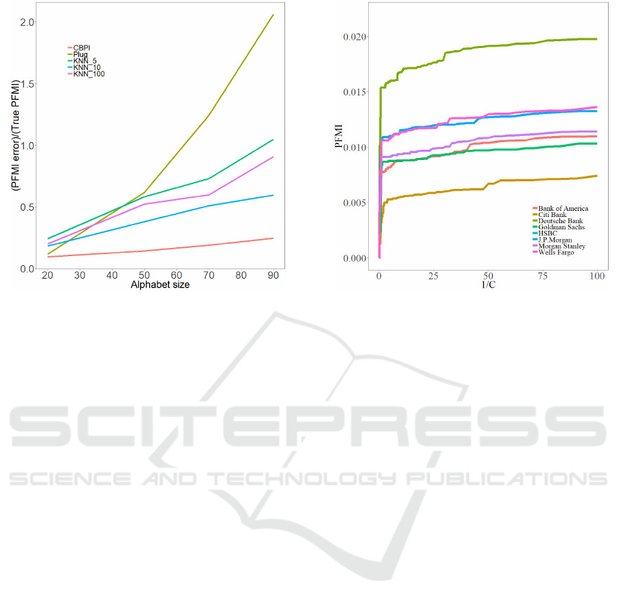
Figure 2: Average PFMI estimation error of the CT-PFMI
algorithm and the benchmark methods with respect to the
true PFMI theoretical value in different values of alphabet
size. The K-NN with different number of neighbors (k) was
calculated using the Parmigene R package (Sales and Ro-
mualdi, 2011).
period of 1.2008-1.2010 that because of the banking
crisis within these years, has a potential of nonzero
{
PFMI in between banks (Dimpfl and Peter, 2014).
The length of the time series was 197,000, hence, a
distributed I/O CT algorithm was implemented.
Stock prices were discretized to `1, 0 and ´1
for positive, zero and negative changes, respectively,
relatively to the price of the previous minute. For
each bank, the PFMI was obtained by implementing
the algorithm of Section 4 for various values of 1{c
(see Fig.3). All curves exhibit a similar behavior of
a phase where uninformative sequences are removed
followed by a steep drop in PFMI after crossing a
certain pruning constant threshold that corresponded
to pruning of sequences from S . The Pruning con-
stant obtained from the CT-PFMI algorithm ranged
between 0.13 to 1.33, depending on the input/output
pair. These values corresponds to filtering 96 percent
of sequences.
Using the descriptive power of the CT-PFMI al-
gorithm, hierarchical analysis can be obtained. For
example, in the higher level, a geographic orientation
can be identified when looking at Fig.3. The esti-
mated PFMI between the European banks HSBC and
DB is higher than the estimated PFMI between these
banks and the American banks.
Moving to lower hierarchies of the interactions,
the conditional probabilities of the output sequences
given the contexts in S differ from the marginal distri-
Figure 3: Estimated PFMI of large banks’ stock prices in the
Wall Street stock exchange (input) with respect to the stock
prices of HSBC bank (output), calculated as a function of
the inverse of the pruning constant c. Shuffled input time
series showed maximum PFMI values of « 5 ¨ 10
´5
.
bution of the output in the probabilities of each sym-
bol, but the symmetry between ´1 and `1 is rela-
tively preserved. For example, see the contexts ob-
tained with the I/O CT of DB to HSBC in Table 1.
Hence, for trading purposes, additional information is
needed.
Another conclusion can be drawn from the con-
texts’ length. The average memory of the process
is 1.5 symbols, as calculated by multiplication of all
contexts’ lengths by their respective probabilities (see
Table 1). This observation implies that most of the
information within τ
p
“ 2.
6 CONCLUSIONS
We showed how the Input/Output context tree algo-
rithm can be utilized to measure the past-future mu-
tual information between time series. Using that,
we demonstrated how the pruning constant param-
eter of the I/O CT algorithm can be calibrated in
a way that separates informative versus uninforma-
tive sequences. This approach constitutes the CT-
PFMI algorithm for PFMI estimation. We used sparse
past-future predictive information (sparse PFMI) sim-
ulated data with a known theoretical PFMI values
to benchmark the CT-PFMI algorithm against other
common PFMI estimation methods. This comparison
shows the advantages of the CT-PFMI algorithm over
the benchmark methods under sparse PFMI condi-
KDIR 2019 - 11th International Conference on Knowledge Discovery and Information Retrieval
70

tions. The CT-PFMI algorithm was also implemented
on real stock prices data to show the sparse PFMI ef-
fect between pairs of real-world time series. It was
also demonstrated how the CT-PFMI algorithm can
be used for in-depth analyses of interactions between
time series.
ACKNOWLEDGEMENTS
This research was funded by the Koret foundation
grant for Smart Cities and Digital Living 2030.
REFERENCES
Begleiter, R., El-Yaniv, R., and Yona, G. (2004). On predic-
tion using variable order markov models. Journal of
Artificial Intelligence Research, 22:385–421.
Begleiter, R., Elovici, Y., Hollander, Y., Mendelson, O.,
Rokach, L., and Saltzman, R. (2013). A fast and
scalable method for threat detection in large-scale dns
logs. In Big Data, 2013 IEEE International Confer-
ence on, pages 738–741. IEEE.
Ben-Gal, I., Morag, G., and Shmilovici, A. (2003). Context-
based statistical process control: A monitoring pro-
cedure for state-dependent processes. Technometrics,
45(4):293–311.
Ben-Gal, I., Shani, A., Gohr, A., Grau, J., Arviv, S.,
Shmilovici, A., Posch, S., and Grosse, I. (2005). Iden-
tification of transcription factor binding sites with
variable-order bayesian networks. Bioinformatics,
21(11):2657–2666.
Bialek, W., Nemenman, I., and Tishby, N. (2001). Pre-
dictability, complexity, and learning. Neural compu-
tation, 13(11):2409–2463.
Bossomaier, T., Barnett, L., Harré, M., and Lizier, J. T.
(2016). An introduction to transfer entropy. Springer.
Brice, P. and Jiang, W. (2009). A context tree method for
multistage fault detection and isolation with applica-
tions to commercial video broadcasting systems. IIE
Transactions, 41(9):776–789.
Chim, H. and Deng, X. (2007). A new suffix tree similarity
measure for document clustering. In Proceedings of
the 16th international conference on World Wide Web,
pages 121–130. ACM.
Cover, T. M. and Thomas, J. A. (2012). Elements of infor-
mation theory. John Wiley & Sons.
Dimpfl, T. and Peter, F. J. (2014). The impact of the fi-
nancial crisis on transatlantic information flows: An
intraday analysis. Journal of International Financial
Markets, Institutions and Money, 31:1–13.
Kaniwa, F., Kuthadi, V. M., Dinakenyane, O., and
Schroeder, H. (2017). Alphabet-dependent parallel al-
gorithm for suffix tree construction for pattern search-
ing. arXiv preprint arXiv:1704.05660.
Kraskov, A., Stögbauer, H., and Grassberger, P. (2004).
Estimating mutual information. Physical review E,
69(6):066138.
Kullback, S. and Leibler, R. A. (1951). On information
and sufficiency. The annals of mathematical statistics,
22(1):79–86.
Kusters, C. and Ignatenko, T. (2015). Dna sequence model-
ing based on context trees. In Proc. 5th Jt. WIC/IEEE
Symp. Inf. Theory Signal Process. Benelux, pages 96–
103.
Largeron-Leténo, C. (2003). Prediction suffix trees for su-
pervised classification of sequences. Pattern Recogni-
tion Letters, 24(16):3153–3164.
Montalto, A., Faes, L., and Marinazzo, D. (2014). Mute: a
matlab toolbox to compare established and novel esti-
mators of the multivariate transfer entropy. PloS one,
9(10):e109462.
Runge, J., Heitzig, J., Petoukhov, V., and Kurths, J. (2012).
Escaping the curse of dimensionality in estimating
multivariate transfer entropy. Physical review letters,
108(25):258701.
Sales, G. and Romualdi, C. (2011). parmigene—a par-
allel r package for mutual information estimation
and gene network reconstruction. Bioinformatics,
27(13):1876–1877.
Satish, U. C., Kondikoppa, P., Park, S.-J., Patil, M., and
Shah, R. (2014). Mapreduce based parallel suffix tree
construction for human genome. In Parallel and Dis-
tributed Systems (ICPADS), 2014 20th IEEE Interna-
tional Conference on, pages 664–670. IEEE.
Schreiber, T. (2000). Measuring information transfer. Phys-
ical review letters, 85(2):461.
Schürmann, T. and Grassberger, P. (1996). Entropy esti-
mation of symbol sequences. Chaos: An Interdisci-
plinary Journal of Nonlinear Science, 6(3):414–427.
Shmilovici, A. and Ben-Gal, I. (2012). Predicting stock re-
turns using a variable order markov tree model. Stud-
ies in Nonlinear Dynamics & Econometrics, 16(5).
Slonim, N., Bejerano, G., Fine, S., and Tishby, N. (2003).
Discriminative feature selection via multiclass vari-
able memory markov model. EURASIP Journal on
Applied Signal Processing, 2003:93–102.
Society, T. X., Wang, S., Jiang, Q., and Huang, J. Z. (2014).
A novel variable-order markov model for clustering
categorical sequences. IEEE Transactions on Knowl-
edge and Data Engineering, 26(10):2339–2353.
Still, S. (2014). Information bottleneck approach to predic-
tive inference. Entropy, 16(2):968–989.
Tishby, N., Pereira, F. C., and Bialek, W. (2000). The
information bottleneck method. arXiv preprint
physics/0004057.
Tiwari, V. S. and Arya, A. (2018). Distributed context tree
weighting (ctw) for route prediction. Open Geospatial
Data, Software and Standards, 3(1):10.
Vicente, R., Wibral, M., Lindner, M., and Pipa, G. (2011).
Transfer entropy—a model-free measure of effective
connectivity for the neurosciences. Journal of compu-
tational neuroscience, 30(1):45–67.
Weinberger, M. J., Rissanen, J. J., and Feder, M. (1995). A
universal finite memory source. IEEE Transactions on
Information Theory, 41(3):643–652.
Yang, J., Xu, J., Xu, M., Zheng, N., and Chen, Y. (2014).
Predicting next location using a variable order markov
model. In Proceedings of the 5th ACM SIGSPATIAL
International Workshop on GeoStreaming, pages 37–
42. ACM.
Past-future Mutual Information Estimation in Sparse Information Conditions
71
