Two New Mutation Techniques for Cartesian Genetic Programming
Roman Kalkreuth
Department of Computer Science, TU Dortmund University, Otto-Hahn-Straße 14, Dortmund, Germany
Keywords:
Cartesian Genetic Programming, Mutation, Phenotype.
Abstract:
Cartesian Genetic Programming is often used with a point mutation as the sole genetic operator. In this
paper, we propose two phenotypic mutation techniques and take a step towards advanced phenotypic mutations
in Cartesian Genetic Programming. The functionality of the proposed mutations is inspired by biological
evolution which mutates DNA sequences by inserting and deleting nucleotides. Experiments with boolean
functions problem show a better search performance when the proposed mutations are used. The results of our
experiments indicate that the proposed mutations are beneficial for the use of Cartesian Genetic Programming.
1 INTRODUCTION
Genetic programming (GP) can be described as a
paradigm which opens the automatic derivation of
programs for problem-solving. First work on GP
has been done by Forsyth (1981), Cramer (1985)
and Hicklin (1986). Later work by Koza (1990,
1992, 1994) significantly popularized the field of GP.
GP traditionally uses trees as program representation.
Just over two decades ago Miller, Thompson, Kal-
ganova, and Fogarty presented first publications on
Cartesian Genetic Programming (CGP) —an encod-
ing model inspired by the two-dimensional array of
functional nodes connected by feed-forward wires of
an FPGA device (Miller et al., 1997; Kalganova and
Miller, 1997; Miller, 1999). CGP offers a graph-
based representation which in addition to standard
GP problem domains, makes it easy to be applied to
many graph-based applications such as electronic cir-
cuits, image processing, and neural networks. CGP
has multiple pivotal advantages:
• CGP comprises an inherent mechanism for the
design of simple hierarchical functions. While
in many optimization systems such a mechanism
has to be implemented explicitly, in CGP multiple
feed-forward wires may originate from the same
output of a functional node. This property can be
very useful for the evolution of goal functions that
may benefit from repetitive inner structures.
• The maximal size of encoded solutions is bound,
saving CGP to some extent from “bloat” that is
characteristic to Genetic Programming (GP).
• CGP offers an implicit way of propagating re-
dundant information throughout the generations.
This mechanism can be used as a source of ran-
domness and memory for evolutionary artifacts.
Propagation and reuse of redundant information
have been shown beneficial for the convergence
of CGP. (Kaufmann and Platzner, 2008)
• CGP encodes a directed acyclic graph. This al-
lows to evolve topologies.
In contrast to tree-based GP for which a broad range
of advanced crossover and mutation techniques have
been introduced and investigated, the state of knowl-
edge of advanced mutation techniques in CGP ap-
pears to be relatively poor. This significant lack of
knowledge in CGP has been the major motivation for
our work. Another motivation for our work has been
the introduction of a phenotypic subgraph crossover
technique for CGP by Kalkreuth et al. (2017). The ex-
periments of Kalkreuth et al. showed that the use of
the phenotypic subgraph crossover technique can be
beneficial for the search performance of CGP. In stan-
dard tree-based GP, the simultaneous use of multiple
types of mutation has been found beneficial by Kraft
et al. (1994) and Angeline (1996). In this paper, we
propose two phenotypic mutations for CGP and take a
step towards advanced phenotypic mutations in CGP.
Furthermore, we present comprehensive experiments
with boolean function problems and demonstrate that
our proposed mutation can be beneficial for the use of
CGP. The structure of the paper is as follows: Section
2 describes CGP briefly and surveys previous work
on advanced mutation techniques in CGP. In Section
3 we propose our new mutation techniques. Section 4
82
Kalkreuth, R.
Two New Mutation Techniques for Cartesian Genetic Programming.
DOI: 10.5220/0008070100820092
In Proceedings of the 11th International Joint Conference on Computational Intelligence (IJCCI 2019), pages 82-92
ISBN: 978-989-758-384-1
Copyright
c
 2019 by SCITEPRESS – Science and Technology Publications, Lda. All rights reserved

is devoted to the experimental results and the descrip-
tion of our experiments. In Section 5 we discuss the
results of our experiments. Finally, section 6 gives a
conclusion and outlines future work.
2 RELATED WORK
2.1 Cartesian Genetic Programming
Cartesian Genetic Programming is a form of Genetic
Programming which offers a novel graph-based rep-
resentation. In contrast to tree-based GP, CGP repre-
sents a genetic program via genotype-phenotype map-
ping as an indexed, acyclic, and directed graph. Orig-
inally the structure of the graphs was a rectangular
grid of N
r
rows and N
c
columns, but later work also
focused on a representation with one row. The genes
in the genotype are grouped, and each group refers to
a node of the graph, except the last one which rep-
resents the outputs of the phenotype. Each node is
represented by two types of genes which index the
function number in the GP function set and the node
inputs. These nodes are called function nodes and ex-
ecute functions on the input values. The number of
input genes depends on the maximum arity N
a
of the
function set. The last group in the genotype repre-
sents the indexes of the nodes which lead to the out-
puts. A backward search is used to decode the cor-
responding phenotype. The backward search starts
from the outputs and processes the linked nodes in
the genotype. In this way, only active nodes are pro-
cessed during the evaluation procedure. The number
of inputs N
i
, outputs N
o
, and the length of the geno-
type is fixed. Every candidate program is represented
with N
r
∗ N
c
∗ (N
a
+ 1) + N
o
integers. Even when the
length of the genotype is fixed for every candidate
program, the length of the corresponding phenotype
in CGP is variable which can be considered as a sig-
nificant advantage of the CGP representation. CGP
is traditionally used with a (1+λ) evolutionary algo-
rithm. The new population in each generation con-
sists of the best individual of the previous population
and the λ created offspring. The breeding procedure
is mostly done by a point mutation which swaps genes
in the genotype of an individual in the valid range by
chance. An example of the decoding from genotype
to phenotype is illustrated in Figure 1.
2.2 Advanced Mutation Techniques in
Standard CGP
For an investigation of the length bias and the search
limitation of CGP, a modified version of the point mu-
Genotype
0 1  0 1 2 1 2 2  3
3
Phenotype
+
/
-
OP
IP1
IP2
Function
Lookup Table
Index Function
0
1
2
Addition
Subtraction
Division
Decode
Node
Number
2 3
4
OP
432
0
1
Figure 1: Exemplification of the decoding procedure of a
CGP genotype to its corresponding phenotype for a math-
ematical function. The nodes are represented by two types
of numbers which index the number in the function lookup
table (underlined) and the inputs (non-underlined) for the
node. Inactive function nodes are shown in gray color.
tation has been introduced by Goldman and Punch
(2013). The modified point mutation exactly mutates
one active gene. This so-called single active-gene mu-
tation strategy (SAGMS) has been found beneficial
for the search performance of CGP. The SAGMS can
be seen as a form of phenotypic genetic operator since
it respects only active function genes in the genotype
which are an active part of the corresponding pheno-
type.
Later work by Manfrini et al. (2016) extended
SAGMS to the so-called Biased Single Active Mu-
tation which is based on the idea of analyzing the be-
havior of the genotype during the evolutionary pro-
cess for a given set of problems. With the help of this
analysis, a bias is created in order to help the direct
gene mutation when applied to other problems. The
mutation operator was proposed for digital combina-
tional logic circuit design. The experiments of Man-
frini et al. (2016) showed that the proposed mutation
performed better or equivalent as the traditional point
mutation. In order to reduce the stalling effect in
CGP and to improve the efficiency of the CGP al-
gorithm, Ni et al. (2014) introduced an Orthogonal
Neighbourhood Mutation (ONM) operator. Accord-
ing to Ni et al., the ONN selects four loci as alleles
of gene strings by chance. Afterward, a Four-factor-
three-level orthogonal experiment with local search is
performed. The results of the experiments demon-
strated that the ONM operator is able to reduce the
stalling effect in CGP and to converge the algorithm
more quickly.
Two New Mutation Techniques for Cartesian Genetic Programming
83

GAGA
CTCT
GAGAGA
CTCTCT
GA
CT
Insertion
Deletion
Original sequence
Mutated sequence
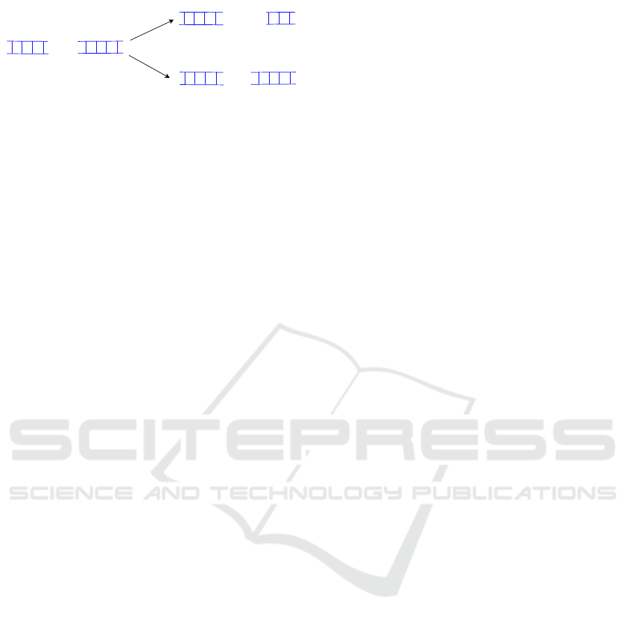
Figure 2: Deletions and insertions of nucleotides.
3 THE PROPOSED METHODS
The proposed mutations for CGP are inspired by bio-
logical evolution in which extra base pairs are inserted
into a new place in the DNA or in which a section of
DNA is deleted. Figure 2 exemplifies the insertion
and deletion mutation on the DNA sequence. Related
to CGP we adopt these so-called frameshift mutations
by activating and deactivating randomly chosen func-
tion nodes. The activation and deactivation of the
nodes are done by adjusting the connection genes of
neighborhood nodes. Both mutation techniques work
similarly as the single active-gene mutation strategy.
The state of exactly one function node in the genome
is changed. Since these forms of mutation can elicit
strong changes in the behavior of the individuals, we
apply an insertion rate and a deletion rate for every
offspring. On the basis of these mutation rates, the
decision is made as to whether the mutations are per-
formed on the genome of an individual. The insertion
and deletion mutation technique work independently
from each other which means that both mutations can
be performed on the genome of the individual in the
breeding procedure of one generation. If the con-
sideration of a minimum or a maximum number of
function nodes is necessary for all individuals in the
population, the algorithms can be parameterized with
maximum and minimum numbers. We will explain
both mutation techniques in detail in the following
two subsections. For both mutation techniques, we
determine the active and passive function nodes of the
respective individual before the mutation procedure.
3.1 The Insertion Mutation Technique
When a genome is selected for the insertion mutation,
one inactive function node becomes active. If all func-
tion nodes are already active or the number of active
function nodes excels a defined maximum, the mu-
tation is rejected. If an individual is suitable for the
insertion mutation, we randomly select one inactive
function node. After the selection we have to distin-
guish three cases:
1. The Selected Inactive Node has a following
Active Function Node.
In this context, the term following function node
means that the node number of an active func-
tion node is greater than the function number of
the randomly selected node. If the selected node
has a following active function node, we copy the
connection genes of the following active node to
the selected inactive node. Afterward, we adjust
one randomly selected connection gene of the fol-
lowing active node to the selected inactive node.
In this way, the selected inactive node will be re-
spected by the backward search and consequently
becomes active. No further steps are required for
the previous active function node since all other
active function nodes remain active due to the
copying of the connection genes.
2. The Selected Inactive Node has a Previous
Active Function Node and no following Active
Function Node.
In this context, the term previous active function
node means that the node number of an active
function node is smaller than the function num-
ber of the randomly selected node. If the selected
node has a previous active function node and no
following active node, at least one output node is
connected with the previous active function node.
In this case, we adjust all output nodes which are
connected with the previous active function node
to the selected inactive node. Afterward, we ad-
just one connection gene of the selected node to
the previous active function node. The other con-
nection genes are randomly connected to previous
active function or input nodes. In this way, the se-
lected inactive node becomes active and the other
inactive function nodes remain inactive.
3. The Selected Inactive Node has no Previous or
following Active Function Node.
If the selected inactive node has no previous or
following active function node, the individual has
no active function nodes. Consequently, the out-
put nodes are directly connected with an input
node. If this is the case, we adjust at least one out-
put node to the selected inactive node. Afterward,
we randomly connect the connection genes of the
selected inactive node to input nodes. In this way,
the selected node becomes active and other func-
tion nodes remain inactive.
3.2 The Deletion Mutation Technique
In contrast to the insertion mutation technique, when
a genome is selected for deletion mutation, one active
node becomes inactive. If all function nodes are inac-
tive or the number of active function nodes is smaller
ECTA 2019 - 11th International Conference on Evolutionary Computation Theory and Applications
84

0 2 1
*
*
+
2
4
4
x
1
6
3  2  2
5
3
/
0
1
5
OP1
2 0  1 
2 0  0
OP1
3
2
0 4  5
6
Parent
Mutant
Insertion
Parent
+
6
0 3 1
4
6
3  2  2
5
2 2 1 
2 0  0
OP1
3
2
0 4  5
6
Mutant
Insertion
*
*
+
4
x
1
3
/
1
5
OP1
+
6
Selected inactive node
0
Node number
Adjusted edges
2
Figure 3: The proposed insertion mutation technique.
0  2  1
*
+
2
4
x
1
6
3  3  3
/
0
1
5
OP1
2 1  0 2 1  0
OP1
0 4  5
Parent
Parent
+
6
0 3 1 6
3  3  3 2 1 0 
2 0  0
OP1
0 4  5
Mutant
Deletion
Mutant
Deletion
*
+
2
4
x
1
/
0
1
5
OP1
+
6
Selected active node
Adjusted edge
Node number
3
4
5
6
2
*
2
3
4
5
6
*
3
3
Figure 4: The proposed deletion mutation technique.
than a defined minimum, the mutation is rejected. If
an individual is suitable for the deletion mutation, we
select the first active function node of the individual.
The deletion mutation procedure is then done by
performing the following steps:
a. Adjust the Connection Genes of All following
Active Function Nodes.
The connection genes of all following active func-
tion nodes which are connected with the selected
active function node are randomly adjusted to
other active function or input nodes.
b. Adjust the Outputs Nodes.
All output nodes which are connected with the
selected active function nodes are randomly ad-
justed to other active function or input nodes.
After performing the adjustment of connection genes
and output nodes, the selected active function node
becomes inactive.
Figure 3 exemplifies the insertion technique. As
visible, one inactive node is selected for activation.
The connection genes in the genotype are adjusted to
activate the selection function node in the phenotype.
In contrast, Figure 4 illustrates an example of a dele-
tion mutation in one active node becomes inactive by
adjusting the respective connection genes. In both fig-
ures, the genotype is grouped into a number of genes
which represent the function and output nodes. More-
over, active function nodes are highlighted in solid
boxes and inactive nodes are shown in dashed boxes.
The selected active or inactive nodes are highlighted
in red.
4 EXPERIMENTS
4.1 Experimental Setup
We performed experiments with boolean function
problems. To evaluate the search performance of the
insertion and deletion mutation techniques, we mea-
sured the number of fitness evaluations until the CGP
algorithm terminated (evaluations-to-termination). In
addition to the mean values of the measurements, we
calculated the standard deviation (SD) and the stan-
dard error of the mean (SEM). We also calculated the
median and the first and second quartile. We per-
formed 100 independent runs with different random
seeds. We used the well known (1 + 4)-CGP algo-
rithm for all experiments. Moreover, we used the
standard CGP point mutation operator in combina-
tion with the insertion and deletion mutations. We
used minimizing fitness functions in all experiments
which are explained in the respective subsection. To
classify the significance of our results, we used the
Mann-Whitney-U-Test. The mean values are denoted
a
†
if the p-value is less than the significance level 0.05
and a
‡
if the p-value is less than the significance level
0.01 compared to the use of the point mutation as the
sole genetic operator.
4.2 Search Performance Evaluation
To evaluate the search performance of the insertion
and deletion mutation techniques, we chose the five
Even-Parity problems with n = 3, 4, 5, 6 and 7
boolean inputs. The goal was to find a program that
produces the value of the boolean even parity depend-
ing on the n independent inputs. The fitness was rep-
resented by the number of fitness cases for which the
candidate solution failed to generate the correct value
of the even parity function.
Since former work by White et al. (2013) outlined
that this problem type was excessively used and inves-
Two New Mutation Techniques for Cartesian Genetic Programming
85

Table 1: Boolean function problems for the search perfor-
mance evaluation.
Problem Number Number
of Inputs of Outputs
Parity-3 3 1
Parity-4 4 1
Parity-5 5 1
Parity-6 6 1
Parity-7 7 1
Adder 1-Bit 3 2
Adder 2-Bit 5 3
Adder 3-Bit 7 4
Multiplier 2-Bit 4 4
Mulitplier 3-Bit 6 6
Demultiplexer 3:8-Bit 3 8
Comparator 4x1-Bit 4 18
Table 2: Configuration of the 1 + 4-CGP algorithm.
Property Value
µ 1
λ 4
Number of nodes 100
Maximum generations 20000000
Function set AND, OR, NAND, NOR
Point mutation rate 4%
Table 3: Insertion and deletion rates for the (1 +4)-CGP-ID
algorithm.
Problem Point mutation Insertion Deletion
rate [%] rate [%] rate [%]
Parity-3 2,5 40 25
Parity-4 1,5 7,5 5
Parity-5 1 8 2
Parity-6 1 6 4
Parity-7 1 6 3
Adder 1-Bit 2 5 5
Adder 2-Bit 1 10 10
Adder 3-Bit 1 5 5
Multiplier 2-Bit 2 5 5
Multiplier 3-Bit 1 6 3
Demultiplexer 3:8-Bit 2 10 10
Comparator 4x1-Bit 1 5 5
tigated in the past, we also evaluated multiple output
problems as the digital adder, multiplier, and demulti-
plexer. These types of problems differ markedly from
the parity problems, and the 3-Bit digital multiplier
has been proposed as a suitable alternative. As a re-
sult, we receive a diverse set of problems in this prob-
lem domain. The set of benchmark problems with the
corresponding number of inputs and outputs is shown
in Table 1. To evaluate the fitness of the individuals on
the multiple output problems, we defined the fitness
value of an individual as the number of different bits
to the corresponding truth table. In order to find per-
formant configurations for the insertion and deletion
mutation rates, we used automated parameter tuning.
The evolved configurations are shown in Table 3.
We compared the (1 + 4)-CGP algorithm to our
modified (1+4)-CGP algorithm equipped with the in-
sertion and deletion mutation techniques. Our modi-
fied (1 + 4)-CGP is denoted as (1 + 4)-CGP-ID. The
number of function nodes was set to 100 for all tested
problems. Following conventional wisdom for CGP,
we use a point mutation rate of 4% for the traditional
(1 + 4)-CGP algorithm. The algorithm configuration
of the (1 + 4)-CGP algorithm is shown in Table 2. We
performed the runtime measurement on a computer
with a Intel(R) Core(TM) i7 CPU 930 with 2.80 GHz
and 24 GB of RAM.
Table 4 presents the results of our search perfor-
mance evaluation which shows a reduced number of
generations until the termination criterion triggers for
the (1 + 4)-CGP-ID algorithm. The results also show
that when the (1 + 4)-CGP-ID is used on more com-
plex boolean function problems, the mean runtime of
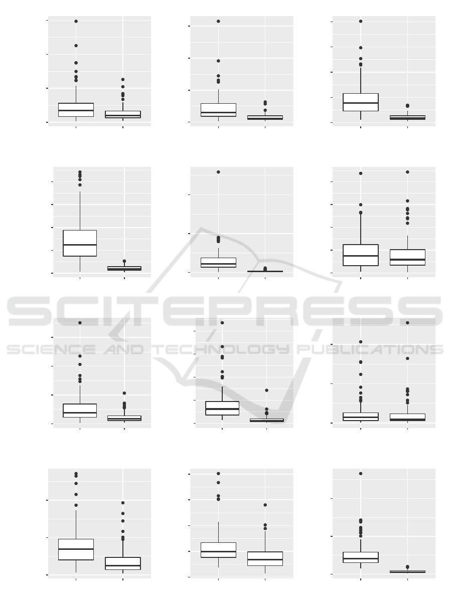
the algorithm is also clearly reduced. Figure 5 pro-
vides boxplots for all tested problems of the search
performance evaluation.
4.3 Comparison to EGGP
We compared three advanced CGP algorithms to a re-
cently introduced method for evolving graphs called
Evolving Graphs by Graph Programming (EGGP).
EGGP has been introduced by Atkinson et al. (2018).
In their experiments, Atkinson et al. compared EGGP
to standard CGP and showed that EGGP performs sig-
nificantly better on the majority of the tested boolean
function problems. Consequently, we chose EGGP
as the baseline for our algorithm comparison. Fur-
thermore, since we evaluated the same set of boolean
function problems as Atkinson et al. we directly
compared the results of our experiments with the re-
sults in Atkinson et al. For our algorithm compar-
ison, we chose the (1 + 4)-CGP-ID algorithm and
also compared EGGP to a (2 + 2)-CGP algorithm
with µ = 2 and λ = 2. The (2 + 2)-CGP algo-
rithm was equipped with the subgraph crossover tech-
nique Kalkreuth et al. (2017). Moreover, we evalu-
ated the (2 + 2)-CGP algorithm with and without the
use of the insertion and deletion technique. In the
presented results, the (2 + 2)-CGP equipped with in-
sertion and deletion mutation is denoted as (2 + 2)-
CGP-ID. We evaluated important parameters like the
crossover and mutation rates empirically. Moreover,
we empirically tuned the parameters µ and λ and
found that a configuration of µ = λ = 2 performs best
on our benchmark problems. The parameter settings
for the crossover and mutation rates of the (2 + 2)-
CGP and (2 + 2)-CGP-ID algorithm are shown in Ta-
ble 5. We measured the number of fitness evalua-
ECTA 2019 - 11th International Conference on Evolutionary Computation Theory and Applications
86

0e+00
1e+04
2e+04
3e+04
(1+4)−CGP (1+4)−CGP−ID
Fitness Evaluations
Parity−3
0e+00
1e+05
2e+05
3e+05
(1+4)−CGP (1+4)−CGP−ID
Parity−4
0e+00
2e+05
4e+05
6e+05
8e+05
(1+4)−CGP (1+4)−CGP−ID
Parity−5
0.0e+00
5.0e+05
1.0e+06
1.5e+06
2.0e+06
(1+4)−CGP (1+4)−CGP−ID
Fitness Evaluations
Parity−6
0e+00
1e+07
2e+07
(1+4)−CGP (1+4)−CGP−ID
Parity−7
0e+00
1e+04
2e+04
3e+04
4e+04
(1+4)−CGP (1+4)−CGP−ID
Adder 1−Bit
0.0e+00
5.0e+05
1.0e+06
1.5e+06
(1+4)−CGP (1+4)−CGP−ID
Fitness Evaluations
Adder 2−Bit
0.0e+00
5.0e+06
1.0e+07
1.5e+07
2.0e+07
(1+4)−CGP (1+4)−CGP−ID
Adder 3−Bit
0e+00
1e+05
2e+05
(1+4)−CGP (1+4)−CGP−ID
Multiplier 2−Bit
0e+00
1e+06
2e+06
(1+4)−CGP (1+4)−CGP−ID
Algorithm
Fitness Evaluations
Multiplier 3−Bit
0e+00
2e+04
4e+04
6e+04
8e+04
(1+4)−CGP (1+4)−CGP−ID
Algorithm
Demultiplexer 3:8−Bit
0e+00
5e+06
1e+07
(1+4)−CGP (1+4)−CGP−ID
Algorithm
Comperator 4x1−Bit
Figure 5: Boxplots for the results of the search performance evaluation.
Two New Mutation Techniques for Cartesian Genetic Programming
87

Table 4: Results of the search performance evaluation.
Problem Algorithm Mean SD SEM 1Q Median 3Q Mean
Fitness Evaluation Runtime
Parity-3
(1 + 4)-CGP 4917 4926 ±493 1695 3412 5598 0.20 s
(1 + 4)-CGP-ID 2700
‡
2173 ±217 1370 1928 3358 0.17 s
Parity-4
(1 + 4)-CGP 43895 43013 ±4301 18125 29398 57968 1.78 s
(1 + 4)-CGP-ID 14381
‡
9905 ±991 8948 11928 19948 1.04 s
Parity-5
(1 + 4)-CGP 194727 148386 ±14839 83304 168996 249993 12.47 s
(1 + 4)-CGP-ID 45349
‡
28257 ±2826 25735 34622 53923 6.99 s
Parity-6
(1 + 4)-CGP 746627 512510 ±51250 371794 617932 937638 112.35 s
(1 + 4)-CGP-ID 105331
‡
52171 ±5217 65445 92466 139067 38.22 s
Parity-7
(1 + 4)-CGP 3074853 3146951 ±314695 1341520 2231156 3696237 976.68 s
(1 + 4)-CGP-ID 283856
‡
177515 ±17751 177610 238426 325776 181.09 s
Adder 1-Bit
(1 + 4)-CGP 9364 8002 ±800 3183 7550 12413 0.23 s
(1 + 4)-CGP-ID 8080
†
7360 ±736 3448 5876 10254 0.23 s
Adder 2-Bit
(1 + 4)-CGP 274734 262394 ±26239 113622 188212 341853 4.98 s
(1 + 4)-CGP-ID 113744
‡
88022 ±8802 56379 84258 140745 3.53 s
Adder 3-Bit
(1 + 4)-CGP 4068492 3567764 ±356776 1802712 3092538 4745253 90.93 s
(1 + 4)-CGP-ID 846075
‡
885420 ±88542 373149 584198 979748 36.39 s
Multiplier 2-Bit
(1 + 4)-CGP 24645 33364 ±3336 6499 14108 26148 0.48 s
(1 + 4)-CGP-ID 21539
‡
33170 ±3317 6372 10196 23753 0.47 s
Multiplier 3-Bit
(1 + 4)-CGP 757523 522412 ±52241 402333 685390 958647 14.60 s
(1 + 4)-CGP-ID 354118
‡
337590 ±33759 142446 250396 465565 9.49s
Demultiplexer 3:8-Bit
(1 + 4)-CGP 23432 13546 ±1355 15258 199918 26750 0.60 s
(1 + 4)-CGP-ID 15523
‡
8994 ±899 8954 13704 19657 0.53 s
Comparator 4x1-Bit
(1 + 4)-CGP 2628085 1848923 ±184892 1528983 2056080 2918599 91.06 s
(1 + 4)-CGP-ID 338019
‡
208523 ±20852 180908 272924 461282 14.65 s
Table 5: Parametrization of the (2 + 2)-CGP and (2 + 2)-
CGP-ID algorithms using subgraph crossover.
Problem Algorithm Crossover Point mut. Insertion Deletion
rate [%] rate [%] rate [%] rate [%]
Parity-3
(2 +2)-CGP 50 4 - -
(2 +2)-CGP-ID 75 1 10 10
Parity-4
(2 +2)-CGP 75 4 - -
(2 +2)-CGP-ID 75 2 20 20
Parity-5
(2 +2)-CGP 75 4 - -
(2 +2)-CGP-ID 75 1 8 2
Parity-6
(2 +2)-CGP 75 4 - -
(2 +2)-CGP-ID 50 1 6 3
Parity-7
(2 +2)-CGP 50 4 - -
(2 +2)-CGP-ID 50 1 6 3
Adder 1-Bit
(2 +2)-CGP 25 4 - -
(2 +2)-CGP-ID 50 2 7,5 7,5
Adder 2-Bit
(2 +2)-CGP 25 4 - -
(2 +2)-CGP-ID 50 1 10 10
Adder 3-Bit
(2 +2)-CGP 25 4 - -
(2 +2)-CGP-ID 50 1 10 5
Multiplier 2-Bit
(2 +2)-CGP 25 4 - -
(2 +2)-CGP-ID 50 2 5 5
Multiplier 3-Bit
(2 +2)-CGP 50 4 - -
(2 +2)-CGP-ID 50 1 6 3
Demultipl. 3:8-Bit
(2 +2)-CGP 25 4 - -
(2 +2)-CGP-ID 75 2 10 10
Comparator 4x1-Bit
(2 +2)-CGP 25 4 - -
(2 +2)-CGP-ID 75 1 5 5
tions until a correct solution was found, similar to our
search performance evaluation. In order to compare
our results directly, we utilized the same evaluation
method as Atkinson et al. by calculating the median
value, the median absolute deviation (MAD) and the
interquartile range (IQR).
Table 6 shows the results of the algorithm com-
parison for all tested boolean function problems. It
is visible that the median values of the (2 + 2)-CGP-
ID and EGGP are on the same level. Moreover, it is
also visible that we achieved a lower median value of
fitness evaluations for the (2 + 2)-CGP-ID algorithm
on some of the tested problems. Please note that the
results for EGGP have been directly taken from the
work of Atkinson et al.
4.4 Fitness Range Analysis
In order to investigate the effects of the insertion and
deletion mutation techniques, we measured the range
of the fitness values for the individuals in the popu-
lation. For the measurement, we defined a budget of
1000 generations for each problem and algorithm. We
measured the range of fitness values in each genera-
tion. At the end of each run, we averaged the mea-
sured range values. Furthermore, we performed 100
runs for each algorithm and problem and averaged the
mean values of each run. With the intention to ensure
generalization in our analysis the (1 + 4)-CGP-ID al-
gorithm was parameterized with a point mutation rate
of 1% and both the insertion and deletion mutation
have been parameterized with a rate of 5%.
Table 7 shows the results of the fitness range anal-
ysis for all tested boolean function problems. As visi-
ble the range of the fitness values of the (1+ 4)-CGP-
ID is much smaller compared to the (1 + 4)-CGP.
Please note, that we used a minimizing fitness func-
tion for our experiments.
ECTA 2019 - 11th International Conference on Evolutionary Computation Theory and Applications
88

Table 6: Results of the algorithm comparison.
Problem Algorithm Median MAD IQR
Parity-3
(1 + 4)-CGP-ID 1928 1578 2052
(2 + 2)-CGP 2778 2986 4564
(2 + 2)-CGP-ID 2203 1318 2098
EGGP 2755 1558 4836
Parity-4
(1 + 4)-CGP-ID 11920 6876 11061
(2 + 2)-CGP 14723 12391 16432
(2 + 2)-CGP-ID 10701 5333 8711
EGGP 13920 5803 11629
Parity-5
(1 + 4)-CGP-ID 34622 21174 28572
(2 + 2)-CGP 128807 83201 105579
(2 + 2)-CGP-ID 27821 14715 25519
EGGP 34368 15190 30054
Parity-6
(1 + 4)-CGP-ID 92466 42247 74034
(2 + 2)-CGP 534039 505962 721456
(2 + 2)-CGP-ID 69742 31376 46839
EGGP 83053 33273 66611
Parity-7
(1 + 4)-CGP-ID 238426 123789 149330
(2 + 2)-CGP 1966944 1558881 2039929
(2 + 2)-CGP-ID 172182 72077 114928
EGGP 197575 61405 131215
Adder 1-Bit
(1 + 4)-CGP-ID 5876 5157 6906
(2 + 2)-CGP 8950 8951 11131
(2 + 2)-CGP-ID 4838 3864 6377
EGGP 5723 3020 7123
Adder 2-Bit
(1 + 4)-CGP-ID 84258 64105 85338
(2 + 2)-CGP 191683 146445 212833
(2 + 2)-CGP-ID 60568 40591 55450
EGGP 74633 32863 66018
Adder 3-Bit
(1 + 4)-CGP-ID 584198 549282 640965
(2 + 2)-CGP 2991999 2379680 3438321
(2 + 2)-CGP-ID 378685 259886 381805
EGGP 275180 114838 298250
Multiplier 2-Bit
(1 + 4)-CGP-ID 10196 17576 17543
(2 + 2)-CGP 17704 20544 19383
(2 + 2)-CGP-ID 7787 10345 10164
EGGP 14118 5553 12955
Multiplier 3-Bit
(1 + 4)-CGP-ID 250396 236555 343552
(2 + 2)-CGP 1024142 777862 993072
(2 + 2)-CGP-ID 166686 118461 196298
EGGP 1241880 437210 829223
Demultiplexer 3:8-Bit
(1 + 4)-CGP-ID 13704 6736 10797
(2 + 2)-CGP 21047 9443 15538
(2 + 2)-CGP-ID 9978 6394 9554
EGGP 16763 4710 9210
Comparator 4x1-Bit
(1 + 4)-CGP-ID 272924 172932 290674
(2 + 2)-CGP 3207723 1788937 3045088
(2 + 2)-CGP-ID 217799 122378 182878
EGGP 262660 84248 174185
4.5 Active Function Node Range
Analysis
With the intention to measure the exploration with
and without our proposed mutation in phenotype
space, we analyzed the range of the active function
nodes. We measured the number of active function
nodes of the best individual in each generation and
calculated the range at the end of each run. The best
individual has a high fitness value and we assume that
the exploration of phenotypes which have a high fit-
ness values is important in order to find the global op-
timum. We performed 100 runs for each algorithm
and allowed a budget of 10000 fitness evaluations.
Afterward, we performed the statistical evaluation on
the range values for the (1+4)-CGP and (1+4)-CGP-
ID algorithm.
Table 8 shows the results of the function node
range analysis for all tested boolean function prob-
lems. It is clearly seen that the range of active func-
tion nodes of the (1 +4)-CGP-ID is greater compared
to the (1 +4)-CGP for the majority of our tested prob-
lems.
Two New Mutation Techniques for Cartesian Genetic Programming
89

Table 7: Results of the fitness range analysis.
Problem Algorithm Mean SD SEM 1Q Median 3Q
Fitness Range
Parity-3
(1 + 4)-CGP 2, 40 0, 43 ±0, 04 2, 06 2, 41 2, 74
(1 + 4)-CGP-ID 1, 50 0, 29 ±0, 029 1, 27 1, 45 1, 71
Parity-4
(1 + 4)-CGP 3, 59 0, 99 ±0, 09 2, 89 3, 62 4, 13
(1 + 4)-CGP-ID 2, 17 0, 64 ±0, 06 1, 75 2, 08 2, 67
Parity-5
(1 + 4)-CGP 3, 88 1, 16 ±0, 11 3, 06 3, 74 4, 54
(1 + 4)-CGP-ID 2, 50 0, 81 ±0, 08 1, 98 2, 45 3, 06
Parity-6
(1 + 4)-CGP 4, 11 1, 60 ±0, 16 2, 91 3, 81 5, 25
(1 + 4)-CGP-ID 2, 90 1, 41 ±0, 14 2, 03 2, 60 3, 45
Parity-7
(1 + 4)-CGP 3, 80 1, 63 ±0, 16 2, 63 3, 59 4, 7
(1 + 4)-CGP-ID 2, 68 1, 54 ±0, 15 1, 62 2, 43 3, 53
Adder 1-Bit
(1 + 4)-CGP 4, 83 0, 59 ±0, 05 4, 46 4, 87 5, 25
(1 + 4)-CGP-ID 2, 61 0, 46 ±0, 04 2, 34 2, 62 2, 94
Adder 2-Bit
(1 + 4)-CGP 16, 50 2, 40 ±0, 24 14, 53 16, 67 17, 86
(1 + 4)-CGP-ID 8, 69 1, 64 ±0, 16 7, 53 8, 55 9, 85
Adder 3-Bit
(1 + 4)-CGP 55, 85 7, 70 ±0, 77 50 55, 97 61, 29
(1 + 4)-CGP-ID 29, 66 5, 82 ±0, 58 25, 57 29, 52 33, 81
Multiplier 2-Bit
(1 + 4)-CGP 13, 48 1, 52 ±0, 15 12, 40 13, 35 14, 41
(1 + 4)-CGP-ID 6, 73 0, 98 ±0, 09 6, 11 6, 75 7, 33
Multiplier 3-Bit
(1 + 4)-CGP 61, 48 5, 48 ±0, 55 58, 11 61, 25 64, 50
(1 + 4)-CGP-ID 28, 47 3, 22 ±0, 32 26, 26 28, 41 30, 50
Demultiplexer 3:8-Bit
(1 + 4)-CGP 11, 07 0, 96 ±0, 10 10, 42 10, 93 11, 53
(1 + 4)-CGP-ID 5, 13 0, 62 ±0, 06 4, 69 5, 06 5, 49
Comparator 4x1-Bit
(1 + 4)-CGP 30, 38 2, 22 ±0, 22 29, 01 30, 21 31, 96
(1 + 4)-CGP-ID 16, 75 1, 65 ±0, 16 15, 65 16, 59 17, 79
5 DISCUSSION
The primary concern of our experiments was to find
significant contributions of the insertion and dele-
tion mutation technique to the search performance of
CGP. The results of our experiments showed benefi-
cial effects on a diverse set of boolean function prob-
lems. One point which should be discussed is the run-
time measurement of our experiments. On one hand,
we observed a reduced amount of fitness evaluations
when the insertion and deletion mutation techniques
were in use for all tested problems. Our runtime
measurement revealed that the beneficial effects were
only significant when the complexity of the problem
is high or when an expensive fitness function is used.
Moreover, the use of the insertion and deletion muta-
tion techniques obviously needs a certain amount of
computational time. However, it is clearly visible that
the use of our proposed mutations showed good run-
time results on the more complex boolean function
problems such as the Parity-7, Adder 3-Bit, and Mul-
tiplier 3-Bit problems. We have to report that we per-
formed our experiments with a naive Java implemen-
tation of both mutation techniques. A more efficient
implementation is left for future work.
Our experiments also addressed the question in
which way the insertion and deletion mutation tech-
niques improve the search performance of CGP. Our
experiments showed that the sole use of the standard
CGP point mutation leads to a wide range of fitness
values. However, when our proposed mutations are
in use, the range of the fitness values is smaller. In
the first place, our results indicate that the sole use
of the point mutation operator is comparatively more
disruptive and can influence the search performance
in a negative way. Moreover, our experiment showed
that the breeding of new individuals is comparatively
less disruptive when our proposed mutations are in
use.
Another part of our experiments was devoted to a
range analysis of the active function node of the best
individual in the population. The results of this exper-
iment indicate that our proposed mutations can lead
to more exploration of the phenotype space. Further-
more, since the best individual is of high fitness, we
assume that the discovery of phenotypes with a high
fitness value is an imporant aspect for the search per-
formance of the CGP algorithm. However, for more
meaningful statements, more detailed analyzes have
to be performed in future work. Our comparison with
EGGP showed that the use of our proposed muta-
tions in combination with the subgraph crossover in-
dicate that these advanced techniques are beneficial
for the use of CGP. Furthermore, on some of our
tested problems, we achieved a lower median value
for the (2 + 2)-CGP-ID algorithm when compared to
EGGP. However, for more significant and meaningful
statements about the current state of EGGP and CGP,
ECTA 2019 - 11th International Conference on Evolutionary Computation Theory and Applications
90

Table 8: Results of the active function node range analysis.
Problem Algorithm Mean Active SD SEM 1Q Median 3Q
Function Node Range
Parity-3
(1 + 4)-CGP 33, 33 4, 54 0, 45 31 33 35
(1 + 4)-CGP-ID 38, 31 7, 82 0, 78 34 39 43
Parity-4
(1 + 4)-CGP 36, 18 3, 97 0, 39 33, 75 36 39
(1 + 4)-CGP-ID 50, 8 6, 04 0, 60 47 51 55
Parity-5
(1 + 4)-CGP 35, 02 4, 13 0, 41 32, 75 34, 75 37
(1 + 4)-CGP-ID 58, 81 5, 17 0, 52 56 59 62
Parity-6
(1 + 4)-CGP 35, 18 4, 52 0, 45 32 34 37, 25
(1 + 4)-CGP-ID 52, 21 6, 73 0, 63 47 53, 5 57
Parity-7
(1 + 4)-CGP 35, 21 4, 27 0, 43 33 35 38
(1 + 4)-CGP-ID 51, 83 6, 80 0, 68 48 51 56, 25
Adder 1-Bit
(1 + 4)-CGP 38, 73 5, 67 0, 56 35 38 42
(1 + 4)-CGP-ID 38, 98 5, 17 0, 52 36 39 42, 25
Adder 2-Bit
(1 + 4)-CGP 36 4, 04 ±0, 40 33 36 38, 25
(1 + 4)-CGP-ID 52, 47 9, 37 ±0, 94 47 52 60
Adder 3-Bit
(1 + 4)-CGP 36, 82 4, 13 0, 41 34 36 39
(1 + 4)-CGP-ID 45, 01 6, 59 0, 66 40 44 49
Multiplier 2-Bit
(1 + 4)-CGP 36.31 3, 81 0, 38 34 36 39
(1 + 4)-CGP-ID 38 4, 95 0, 49 35 37 41
Multiplier 3-Bit
(1 + 4)-CGP 36, 46 4, 74 0, 47 33 36 39
(1 + 4)-CGP-ID 41, 28 5, 47 0, 55 37 40, 5 46
Demultiplexer 3:8-Bit
(1 + 4)-CGP 35, 53 4, 16 0, 42 32, 75 35 38
(1 + 4)-CGP-ID 42, 69 6, 00 0, 60 39 42 46, 25
Comparator 4x1-Bit
(1 + 4)-CGP 30, 38 3, 53 0, 35 28 30 33
(1 + 4)-CGP-ID 32, 6 5, 40 0, 54 29 32 36
a more comprehensive study is needed and should
include different problem domains. For the field of
graph-based Genetic Programming, this point is of
high importance because there is comparatively only
a little knowledge about the search performance of
CGP and EGGP in other problems domains. More-
over, EGGP and CGP have been mostly evaluated
with boolean function problems in the past which re-
sulted in a one-sided state of knowledge. Therefore,
we think that comprehensive comparative studies are
needed to expand the current state of knowledge.
Addressing the reasons of the effectiveness of the
(2 + 2)-CGP-ID algorithm, we have to acknowledge
that we don’t have any results and answers to the
question in which way the combination of subgraph
crossover and our proposed mutations contribute to
the search performance of CGP. The results of our ex-
periments open two questions which have to be tack-
led with our future work: In the first place we have to
find answers in which way the (2 + 2)-CGP-ID algo-
rithm contributes to the search performance of CGP.
In order to achieve insight into the detailed functional
mechanism of the (2 + 2)-CGP and (2 + 2)-CGP-ID
algorithm, we have to understand the proposed meth-
ods in detail. As a first step forward, we think a sep-
arate investigation of exploitation and exploration ef-
fects of the (2 + 2)-CGP and (2 + 2)-CGP-ID algo-
rithm would be helpful. We also have to tackle the
question of why small population sizes are generally
successful in the Boolean domain. Since the effective-
ness of the (1 +4)-CGP in the boolean domain is well
known in the field of CGP (Miller, 1999; Miller and
Smith, 2006), our experiments with the (2 + 2)-CGP-
ID algorithm underline the effectiveness of small pop-
ulation sizes in the boolean problem domain. Conse-
quently, there is a need for more insight into the ob-
served conditions of our experiments.
6 CONCLUSION AND FUTURE
WORK
Within this paper, we proposed two new phenotypic
mutation techniques and took a step towards advanced
phenotypic mutations in CGP. The results of our ex-
periments clearly show that our proposed methods
can be beneficial for the use of CGP. Our experiments
also clearly show that the insertion and deletion mu-
tation techniques can significantly improve the search
performance of CGP. We also compared CGP to an-
other state-of-the-art method for evolving graphs and
showed that advanced methods of crossover and mu-
tation allow CGP to perform well.
The analytic part of our experiments showed on
one hand that the sole use of the point mutation op-
erator in CGP can cause more disruptive effects com-
pared to the use of our proposed mutations in com-
bination with the point mutation operator. Moreover,
our experiments indicate that our proposed mutations
enable a wider search in high fitness regions within
the search space. For more significant statements
Two New Mutation Techniques for Cartesian Genetic Programming
91

about the beneficial effects of the proposed mutations,
a rigorous and comprehensive study on a larger set
of problems is needed and should include the inves-
tigation of different problem domains. Consequently,
we will mainly focus on more detailed and compre-
hensive experiments in the future including other GP
problem domains. These experiments will also in-
clude an analysis of the exploration abilities of CGP
when the proposed mutations are in use. Another
part of our future work is devoted to a detailed inves-
tigation of the (2 + 2)-CGP-ID algorithm with sub-
graph crossover and our mutations. This will also
include an investigation in which way the subgraph
crossover and our proposed mutations work together
and if there are similar functional behaviors between
different problems. This part of our future work has
to address the question of the effectiveness of small
population sizes in the boolean domain. The last point
for our future work is the application of our proposed
mutation techniques to other GP representations.
REFERENCES
Angeline, P. J. (1996). An investigation into the sensitiv-
ity of genetic programming to the frequency of leaf
selection during subtree crossover. In Koza, J. R.,
Goldberg, D. E., Fogel, D. B., and Riolo, R. L., ed-
itors, Genetic Programming 1996: Proceedings of the
First Annual Conference, pages 21–29, Stanford Uni-
versity, CA, USA. MIT Press.
Atkinson, T., Plump, D., and Stepney, S. (2018). Evolving
graphs by graph programming. In Castelli, M., Sekan-
ina, L., Zhang, M., Cagnoni, S., and Garcia-Sanchez,
P., editors, EuroGP 2018: Proceedings of the 21st Eu-
ropean Conference on Genetic Programming, volume
10781 of LNCS, pages 35–51, Parma, Italy. Springer
Verlag.
Cramer, N. L. (1985). A representation for the adaptive gen-
eration of simple sequential programs. In Proceedings
of the 1st International Conference on Genetic Algo-
rithms, pages 183–187, Hillsdale, NJ, USA. L. Erl-
baum Associates Inc.
Forsyth, R. (1981). Beagle — a darwian approach to pattern
recognition. Kybernetes, 10(3):159–166.
Goldman, B. W. and Punch, W. F. (2013). Length bias
and search limitations in cartesian genetic program-
ming. In Proceedings of the 15th Annual Conference
on Genetic and Evolutionary Computation, GECCO
’13, pages 933–940, New York, NY, USA. ACM.
Hicklin, J. (1986). Application of the genetic algorithm to
automatic program generation. Master’s thesis.
Kalganova, T. and Miller, J. F. (1997). Evolutionary Ap-
proach to Design Multiple-valued Combinational Cir-
cuits. In Proc. Intl. Conf. Applications of Computer
Systems (ACS).
Kalkreuth, R., Rudolph, G., and Droschinsky, A. (2017).
A new subgraph crossover for cartesian genetic pro-
gramming. In Castelli, M., McDermott, J., and Sekan-
ina, L., editors, EuroGP 2017: Proceedings of the
20th European Conference on Genetic Programming,
volume 10196 of LNCS, pages 294–310, Amsterdam.
Springer Verlag.
Kaufmann, P. and Platzner, M. (2008). Advanced tech-
niques for the creation and propagation of modules
in cartesian genetic programming. In Proceedings of
the 10th Annual Conference on Genetic and Evolu-
tionary Computation, GECCO ’08, pages 1219–1226,
New York, NY, USA. ACM.
Koza, J. (1990). Genetic Programming: A paradigm for ge-
netically breeding populations of computer programs
to solve problems. Technical Report STAN-CS-90-
1314, Dept. of Computer Science, Stanford Univer-
sity.
Koza, J. R. (1992). Genetic Programming: On the Pro-
gramming of Computers by Means of Natural Selec-
tion. MIT Press, Cambridge, MA, USA.
Koza, J. R. (1994). Genetic Programming II: Automatic
Discovery of Reusable Programs. MIT Press, Cam-
bridge Massachusetts.
Kraft, D. H., Petry, F. E., Buckles, B. P., and Sadasivan,
T. (1994). The use of genetic programming to build
queries for information retrieval. In Proceedings of the
1994 IEEE World Congress on Computational Intelli-
gence, volume 1, pages 468–473, Orlando, Florida,
USA. IEEE Press.
Manfrini, F. A. L., Bernardino, H. S., and Barbosa, H. J. C.
(2016). A novel efficient mutation for evolutionary de-
sign of combinational logic circuits. In Handl, J., Hart,
E., Lewis, P. R., L
´
opez-Ib
´
a
˜
nez, M., Ochoa, G., and
Paechter, B., editors, Parallel Problem Solving from
Nature – PPSN XIV, pages 665–674, Cham. Springer
International Publishing.
Miller, J. F. (1999). An empirical study of the efficiency
of learning boolean functions using a cartesian ge-
netic programming approach. In Proceedings of the
Genetic and Evolutionary Computation Conference,
volume 2, pages 1135–1142, Orlando, Florida, USA.
Morgan Kaufmann.
Miller, J. F. and Smith, S. L. (2006). Redundancy and com-
putational efficiency in cartesian genetic program-
ming. IEEE Transactions on Evolutionary Computa-
tion, 10(2):167–174.
Miller, J. F., Thomson, P., and Fogarty, T. (1997). De-
signing Electronic Circuits Using Evolutionary Algo-
rithms. Arithmetic Circuits: A Case Study.
Ni, F., Li, Y., Yang, X., and Xiang, J. (2014). An orthogonal
cartesian genetic programming algorithm for evolv-
able hardware. In 2014 International Conference on
Identification, Information and Knowledge in the In-
ternet of Things (IIKI), pages 220–224.
White, D. R., McDermott, J., Castelli, M., Manzoni, L.,
Goldman, B. W., Kronberger, G., Jaskowski, W.,
O’Reilly, U.-M., and Luke, S. (2013). Better GP
Benchmarks: Community Survey Results and Propos-
als. Genetic Programming and Evolvable Machines,
14(1):3–29.
ECTA 2019 - 11th International Conference on Evolutionary Computation Theory and Applications
92