
Genetic Algorithm with Success History based Parameter Adaptation
Vladimir Stanovov
a
, Shakhnaz Akhmedova
b
and Eugene Semenkin
c
Reshetnev Siberian State University, Krasnoyarskii rabochii ave. 31, 660037, Krasnoyarsk, Russian Federation
Keywords:
Genetic Algorithm, Optimization, Parameter Control, Metaheuristic, Simulated Binary Crossover.
Abstract:
Genetic algorithm is a popular optimization method for solving binary optimization problems. However,
its efficiency highly depends on the parameters of the algorithm. In this study the success history adaptation
(SHA) mechanism is applied to genetic algorithm to improve its performance. The SHA method was originally
proposed for another class of evolutionary algorithms, namely differential evolution (DE). The application
of DE’s adaptation mechanisms for genetic algorithm allowed significant improvement of GA performance
when solving different types of problems including binary optimization problems and continuous optimization
problems. For comparison, in this study, a self-configured genetic algorithm is implemented, in which the
adaptive mechanisms for probabilities of choosing one of three selection, three crossover and three mutation
types are implemented. The comparison was performed on the set of functions, presented at the Congress on
Evolutionary Computation for numerical optimization in 2017. The results demonstrate that the developed
SHAGA algorithm outperforms the self-configuring GA on binary problems and the continuous version of
SHAGA is competetive against other methods, which proves the importance of the presented modification.
1 INTRODUCTION
The development of modern and efficient optimiza-
tion methods is an important direction of research, be-
cause these methods could find their application in the
area of various technical, engineering and scientific
problems. Today, heuristic methods, which do not
use any information about specific properties of the
problem at hand, have gained a lot of attention from
the research community as they are capable of solv-
ing any type of optimization problems, including bi-
nary, integer, real-valued, combinatorial, constrained,
multi-objective optimization problems and many oth-
ers.
One of the earliest heuristic methods is the Ge-
netic Algorithm (GA), which uses the idea of natu-
ral evolution to generate new solutions via operators
of selection, crossover, mutation and population up-
date. Modern genetic algorithms usually rely on a
set of different types of genetic operators, mentioned
above, and many of them implement self-adaptation
or self-configuration schemes. The self-configuration
is required because the efficiency of GA depends on
the type of operators used: each operator has its own
a
https://orcid.org/0000-0002-1695-5798
b
https://orcid.org/0000-0003-2927-1974
c
https://orcid.org/0000-0002-3776-5707
properties, which could be helpful at different stages
of the search process. Moreover, some genetic algo-
rithm variants use parameter adaptation mechanisms
to change the probabilities of selection, crossover and
mutation operators’ application, for example, (Eiben
et al., 1999), (Semenkin and Semenkina, 2012a), (Se-
menkin and Semenkina, 2012b).
Modern GA versions rely on self-configuration
schemes, developed specifically for GA, however,
there are many other evolutionary techniques which
have their own adaptation schemes. For example,
many Differential Evolution (DE) variants use the
Success History Adaptation (SHA) scheme to tune
numerical parameters, first presented in (Tanabe and
Fukunaga, 2013). Although this adaptation method
is meant to be used only for DE, its efficiency was
proved many times (Al-Dabbagh et al., 2018), and
with small modifications it could be used for GA.
In this study the genetic algorithm is designed fol-
lowing the scheme of DE, and with SHA method.
The computationalexperimentsshowthe efficiencyof
such modification, both on binary and real-valued op-
timization problems, compared to the self-configured
GA.
The rest of the paper is organized as follows: sec-
tion 2 describes the basics of GA and known self-
configuration schemes, section 3 presents the SHA
180
Stanovov, V., Akhmedova, S. and Semenkin, E.
Genetic Algorithm with Success History based Parameter Adaptation.
DOI: 10.5220/0008071201800187
In Proceedings of the 11th International Joint Conference on Computational Intelligence (IJCCI 2019), pages 180-187
ISBN: 978-989-758-384-1
Copyright
c
2019 by SCITEPRESS – Science and Technology Publications, Lda. All rights reserved

method and GA implementation, section 4 includes
experimental setup and results, and section 5 con-
cludes the paper.
2 GENETIC ALGORITHM AND
SELF-CONFIGURATION
The genetic algorithm relies on a population of so-
lutions, each encoded as a string or chromosome of
binary values, i.e. 0 or 1. Each individual represents a
potential solution to the problem at hand, and may en-
code any characteristics of the solution, including nu-
merical values, structural chraracteristics, choice be-
tween alternatives and so on. The population devel-
ops towards better solutions,according to the defined
fitness function, defined by the goal function, via par-
ents selection, their crossover to produce offspring,
random mutation and replacement of parents with off-
spring.
The selection mechanism is used to define which
individuals will transfer their genetic information to
the next generation. All selection mechanisms de-
termine the probability values (in explicit or implicit
way) for every individual in the population to be cho-
sen. The three most popular selection schemes are:
proportional selection, rank-based selection and tour-
nament selection (Goldberg and Deb, 1991).
In proportinal selection the probability of an indi-
vidual is directly proportionalto its normalized fitness
value, so that individuals with better fitness get higher
probabilities. The disadvantages of proportinal selec-
tion are premature convergence and super-individual
problem. The rank-based selection assigns probabil-
ities based on the rank of the individual in the array
sorted by fitness - this method allows eliminating the
disadvantages of proportional selection. The tourna-
ment selection does not explicitly calculate probabili-
ties, instead each individual is chosen as a winner in a
tournament of t randomly selected individuals in the
population. In (Stanovov et al., 2018) it was shown
that in case if t = 2, the probability of selection is the
same as for rank-based selection with linear rank as-
signment.
The crossover is used to mix the genetic informa-
tion of parents, without introducing any new infor-
mation. Popular crossover methods in GA are: one-
point, two-point and uniform crossover. In one point
crossover, a single point in the cromosome is chosen
and the binary strings exchange their tails. In two-
point crossover, two points are chosen and individuals
exchange the middle part. In uniform crossover, every
bit can be chosen from either one parent or another.
There are usually several levels of mutation prob-
abilities used in GA, referred to as weak, average and
strong mutation. In average mutation the probabil-
ity of a bit j being flipped is p
m
ut =
1
L
, where L is
the length of the binary string encoding the solution.
Weak mutation changes the probability to be 3 times
less then average, while strong mutation increases p
j
by 3 times.
The self-configuration method used in (Semenkin
and Semenkina, 2012a) and (Semenkin and Semenk-
ina, 2012b) is based on the idea of selecting one of
the three types of selection, crossover and mutation
depending on their efficiency at the moment. Initially
all probabilities are set to p
i
=
1
z
, where z is the num-
ber of different operators (3 in this study) of a certain
type. The efficiency is measured as the average fitness
at current generation:
AvgFit
i
=
∑
n
i
j=1
f
i, j
n
i
, i = 1, 2, ...z (1)
where n
i
is the number of offspring, created with i-
th operator, f
i, j
is the fitness if j-th offspring, cre-
ated with i-th operator, AvgFit
i
is the average fitness
of individuals created with i-th operator. Based on
the AvgFit
i
values, the winning operator w of each
type is defined, and is probability is increased by
p
w
= p
w
+
(z−1)K
zN
, and the probabilities of other op-
erators are decreased by
K
zN
, where K is a constant,
set to 0.5 and N is the population size. Also, for all
operators the minimal level of p
i
was set to 0.05.
This probabilities tuning method was shown to
perform better than GA with randomly chosen oper-
ator types among variety of problems, but still worse
then the best combination of selection, crossover and
mutation for a particular problem, which was defined
by extensive numerical experiments. Further in the
text the described self-configuring binary GA will be
reffered to as SelfCGA.
In case of continous optimization problems, usu-
ally special versions of crossover and mutation op-
erators are used, most popular are simulated binary
crossover (SBX) (Deb and Agrawal, 1995) and poly-
nomial mutation (Deb and Deb, 2014). The SBX op-
erator searches for solutions in real-parameter space
in a manner similar to single-point crossover, and
polynomial mutation applies polinomial distribution
to search for solutions next to an individual. In the
next section, the success history adaptation is pre-
sented, as well as its application to GA crossover and
mutation operators.
Genetic Algorithm with Success History based Parameter Adaptation
181

3 PROPOSED APPROACH:
GENETIC ALGORITHM WITH
SUCCESS HISTORY
ADAPTATION
The success history adaptation mechanism was origi-
nally proposed to adjust the numerical values of scal-
ing factor F and crossover rate Cr in differential evo-
lution. This tuning mechanism is based on an earlier
study, which was introduced in the JADE algorithm,
(Zhang and Sanderson, 2009), where the successful
values of F and Cr were used to define new values.
In SHA there are H memory cells, each containing
a set of parameters. In this study for binary GA there
are two tuned parameters: the mutation rate Mr and
crossover rate Cr were tuned, so that each k-th mem-
ory cell is denoted as M
Mr,k
and M
Cr,k
. The initial
value for M
Mr,k
is set to
3
L
, maximum value -
5
L
, and
M
Cr,k
is initially set to 0.5. For every individual in the
population, a random memory cell index i is chosen,
and the new Mr is sampled with Cauchy distribution
(scale parameter 0.1), while Cr is sampled with nor-
mal distribution (standard deviation 0.1) as follows:
Mr = randc(M
Mr,i
, 0.1), Cr = randn(M
Cr,i
, 0.1) (2)
After each application of crossover and mutation,
if there was an improvement in fitness value, success-
ful Mr and Cr values are saved to S
Mr
and S
Cr
respec-
tively. At the end of the generation, h-th memory cell
is updated with new values, calculated using weighted
Lehmer mean:
mean
wL
(S) =
∑
|S|
j=1
w
j
S
2
j
∑
|S|
j=1
w
j
S
j
(3)
where S could be S
Mr
or S
Cr
, w
j
=
∆f
j
∑
|S|
k=1
∆f
k
, ∆f
j
=
| f(x
new
) − f(x
old
)|. The index number h is incre-
mented in a loop every generation, and if h = H, h
is set to 1.
The crossover rate Cr is limited to [0, 1], and mu-
tation rate Mr - to [0,
5
L
]. In this manner, the SHA
adaptation mechanism identifies the best parameter
values at current generation not only depending on
which values were mostly successful, but also taking
into consideration the improvement level ∆ f
The rest of the GA scheme is also changed to be
similar to DE scheme. At every generation, for ev-
ery i-th individual the second parent is selected with
tournament selection, tournament size t = 2. Next, i-
th individual and selected individual are combined in
uniform crossover operator, where Cr = 1 means that
all genetic information will be taken from the new in-
dividual - all L bits of the selected individual have
100% chance to be chosen. Also, to make sure that
at least some information is taken from the selected
individual, one randomly selected bit is copied from
the selected individual. Next, at the mutation step ev-
ery bit in the newly created individual after crossover
is flipped with probability Mr. There could be situ-
ations when no bits are changed, or all of them are
changed, but the last is highly improbable.
After mutation, the replacement scheme is ap-
plied. The newly generated individual, modified in
crossover and mutation, is compared to the i-th indi-
vidual in the population. If there is an improvement
in fitness value, the i-th individual is replaced, and Mr
andCr are saved. Otherwise, no actions are taken, and
the algorithm proceeds to the next individual. The de-
scribed algorithm was called SHAGA, and tested to
compare with the self-configuring GA in section 2.
For the case of continous optimization, there
were 4 tuned parameters, including crossover rate
Cr in range [0, 1], mutation rate Mr in range [0,
3
D
],
crossover distribution index η
c
in range [10, 200] and
mutation distribution index η
m
in range [10, 200]. The
tournament size was also set to t = 2, crossover was
performed between the i-th individual and selected in-
dividual, and the replacement occured only if the gen-
erated trial individual was at least as good as the first
parent.
The next section describes the experimental setup
and the results of algorithm comparison.
4 EXPERIMENTAL SETUP AND
RESULTS
The efficiency of the newly designed SHAGA algo-
rithm was tested on binary and numerical optimiza-
tion problems. Two classical binary problems were
selected for experiments, namely the onemax prob-
lem and 01 problem. For onemax problem, the goal
is to set all bits to 1, and for 01 problem the goal is to
find a string with maximum number of ”01” combi-
nations in it. The first problem has only one optima,
while the 01 problem has one local optima and one
global optima, which differ by a shift by one bit.
The experiments for these binary problems were
performed for the length of binary string of 100, 1000
and 3000. The amount of computational resource was
the same for both SHAGA and SelfCGA: for 100 bits
the maximum number of fucntion evaluations was set
to NFE = 10
4
, for 1000 bits NFE = 10
5
, for 3000
bits NFE = 10
6
. The population size was set to 100,
100 and 1000 respectively.
To track the convergence process for every of the
30 indepenent runs of the algorithm, the best achieved
ECTA 2019 - 11th International Conference on Evolutionary Computation Theory and Applications
182
fitness value was saved after 0.01, 0.02, 0.03, 0.05,
0.1, 0.2, 0.3, 0.4, 0.5, 0.6, 0.7, 0.8, 0.9 and 1.0 frac-
tions of the maximum number of function evaluations
NFE
max
. The comparison of the final results was
performed with two-tailed Mann-Whitney rank sum
statistical test with tie braking and significance level
p = 0.01.
Firstly, the SHAGA with fixed Mr andCr parame-
ters was tested, i.e. Mr =
1
L
, Cr = 0.5. In Figure 1 the
avegaged convergencegraphs of SHAGA without pa-
rameter tuning and SelfCGA are presented. The val-
ues in the graphs are the fitness of individuals, which
is the number of ones for onemax problem, and num-
ber of 01 combinations for 01 problem.
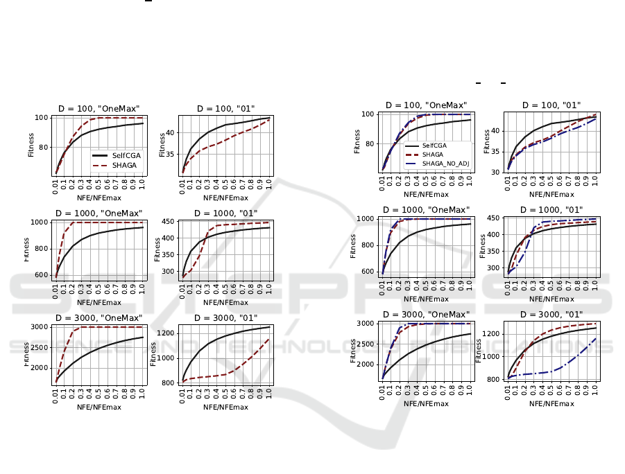
Figure 1: Convergence of SelfCGA and SHAGA with fixed
parameters.
From Figure 1 it could be observed that for bi-
nary string length of 100, for Onemax problem the
convergence of SHAGA and SelfCGA is similar at
the beginning, but later on, at around 0.4NFE
max
the
SHAGA reaches the goal, while SelfCGA fails to
achieve 100 correct bits until the end of the search.
For 01 problem the situation is different, SelfCGA
demonstrates superior performance during the search
process, but SHAGA eventuallty gets the same re-
sult. For the case of D = 1000 SHAGA demon-
strates superior performance for both onemax and 01
problem. However, for 01 problem at the beginning
SelfCGA converges faster, but SHAGA takes over at
0.3NFE
max
. For D = 3000 the behaviour of algo-
rithms is quite different: for 01 problem SelfCGA
converges faster then SHAGA, although it is clearly
seen that SHAGA accelerates its convergence in a
similar way as for D = 100 and D = 1000. Also,
note that SHAGA converges to the optimum for one-
max problem in all cases. According to the Mann-
Whintney statistical test, SHAGA has shown superior
performance in 4 cases out of 6 (all onemax prob-
lems and 01 for D = 1000), and for two other cases
there was no significant difference in algorithms per-
formance. From the graphs it could be seen that with
larger resource SHAGA will probably outperform the
SelfCGA for all 01 problem instances.
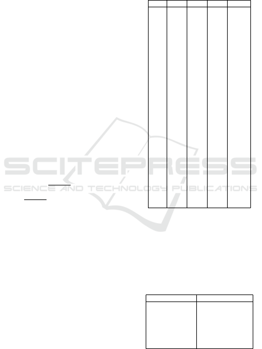
In Figure 2 the results for SelfCGA and SHAGA
with success-history adaptive parameter tuning are
presented. The algorithm without parameter adapta-
tion is denoted as SHAGA
NO ADJ.
Figure 2: Convergence of SelfCGA and SHAGA with pa-
rameter tuning.
From Figure 2 it could be seen that adding param-
eter tuning significantly improves the performance of
SHAGA: convergence on 01 problem in comparison
to the algorithm without parameter tuning is signifi-
cantly faster. This is especially seen for D = 3000,
where SHAGA with success history adaptation out-
performes SelfCGA already after 0.3NFE
max
. As for
onemax problem, there is also a small improvement
for SHAGA. The Mann-Whitney statistical signifi-
cance test indicates superior performance of SHAGA
over SelfCGA in all cases except 01 problem for
D = 100. SHAGA with parameter adaptation is better
then without for D = 100 and D = 3000 for 01 prob-
lem.
The next series of experiments was performed on
a set of benchmark problems from the Congress on
Evolutionary Computation (CEC) 2017 for single-
Genetic Algorithm with Success History based Parameter Adaptation
183
objective real-valued bound-constrained optimiza-
tion. The set of benchmark problems consists of 30
functions defined for dimensions 10, 30, 50 and 100.
These test problems are specifically designed to test
evolutionary optimization techniques, including GA.
The functions are characterized by various properties
that make them difficult to optimize, including many
local optima, non-separability, different properties for
different variables, areas of equal fitness values, i.e.
plateaus, small area of global optima attraction and
others. According to the competition rules, there were
51 independent runs performed for all dimensions and
all 30 test functions, and the difference between the
goal function value and the best achieved value was
recorded. All test problems are minimization func-
tions. To avoid cheating of some algorithms which
check the center of coordinates for optimal solution,
the whole functions were shifted by random value
from the center of coordinates, and all functions were
rotated. The function definition can be found in (Wu
et al., 2016).
First, the binary versions of SHAGA and Self-
CGA were modified to solve numerical optimization
problems in the following manner: each numerical
variable was defined within the range [x
min
, x
max
] with
x
min
= −100, x
max
= 100. For every variable the ini-
tial accuracy of the grid was set to acc = 0.01. Next,
for every i-th variable the minimal length of the bi-
nary string required to encode the grid was calcu-
lated as L
i
= log
2
(
(x
max
−x
min
)
acc
) rounded to the next
integer. After this, the new step was calculated as
acc
new
=
(x
max
−x
min
)
L
. The final string length was the
sum of all L
i
. Both algorithms used the reflected bi-
nary code (Gray encoding) for numerical values. The
population size for both SHAGA and SelfCGA was
set to 350, maximum number of function evaluations
- 10
5
D. Table 1 contains the detailed results of sta-
tistical tests of SelfCGA and SHAGA, where 1 means
that SHAGA was better, -1 that SelfCGA was better,
and 0 means no significant difference.
The results presented in Table 1 demonstrate that
SHAGA is better then SelfCGA for most problems,
and according to Mann-Whitney statistical test, for
D = 10 SHAGA was significantly better for 24 func-
tions out of 30, and worse for 2 functions, namely
F3 and F12. Moreover, SelfCGA was observed to
stagnates sometimes, in particular for F14, F15, F19,
F20, F21, F24, while SHAGA continues search for
all problems. For D = 30 SHAGA demonstrates sta-
tistically significant better results for 23 functions out
of 30. For D = 50 there are 23 improvements out of
30, and for D = 100 - 27 improvements. SHAGA not
only demonstrates better performance for most prob-
lems, but also in some cases converged to the global
Table 1: Statistical test results for SHAGA and SelfCGA,
numerical problems.
Func D=10 D=30 D=50 D=100
f1 1 1 1 1
f2 1 1 1 1
f3 -1 -1 -1 -1
f4 1 -1 -1 1
f5 1 1 1 1
f6 1 1 1 1
f7 1 1 1 1
f8 1 1 1 1
f9 0 1 1 1
f10 1 1 1 1
f11 0 0 0 1
f12 1 1 1 1
f13 1 1 1 0
f14 1 1 1 0
f15 1 0 0 1
f16 1 1 1 1
f17 -1 1 1 1
f18 0 1 1 1
f19 1 0 0 1
f20 1 1 1 1
f21 1 1 1 1
f22 1 1 1 1
f23 1 1 1 1
f24 1 1 1 1
f25 1 0 0 1
f26 1 1 1 1
f27 0 1 1 1
f28 0 1 1 1
f29 1 0 0 1
f30 1 1 1 1
optima, for example for D = 10 for F9, despite of the
discretization of the search space and binary endcod-
ing. Table 2 summs up the statistical tests results
for SHAGA and SelfCGA. In this table ”+” stands
for significant improvement of SHAGA against Self-
CGA, ”-” for significant deterioration in performance,
and ”=” for insignificant difference. For binary case,
there were 2 functions, and 30 functions for numerical
case.
Table 2: Statistical test results for SHAGA and SelfCGA,
numerical problems.
Problem type SHAGA vs SelfCGA
Binary, D=100 1+/0-/1=
Binary, D=1000 2+/0-/0=
Binary, D=3000 1+/0-/1=
Numerical, D=10 23+/2-/5=
Numerical, D=30 23+/0-/7=
Numerical, D=50 23+/2-/5=
Numerical, D=100 27+/1-/2=
ECTA 2019 - 11th International Conference on Evolutionary Computation Theory and Applications
184
In the next series of experiments the continuous
version SHAGA
c
was used, with real-valued param-
eter encoding instead of binary, SBX crossover and
poynomial mutation as described above. First, the
efficiency of the parameter adaptation scheme was
tested, for this the GA
c
(without SHA) was tested with
the following fixed parameters: Cr = 0.5, Mr =
1
D
,
η
c
= 50, η
m
= 50. The population size was set to
10D, the computational resource was set to 10000D.
Table 3 contains statistical test results for SHAGA-c
with GA-c.
Table 3: Statistical test results for SHAGA
c
and GA
c
.
Problem type SHAGA
c
and GA
c
D=10 13+/16-/1=
D=30 25+/4-/1=
D=50 24+/6-/1=
D=100 22+/7-/1=
In Table 3 ”+” stands for significant improvement
of SHAGA-c againstGA-c, ”-” for significant deterio-
ration in performance, and ”=” for insignificant differ-
ence. Except for D = 10, the SHA allowed significant
improvement of performance.
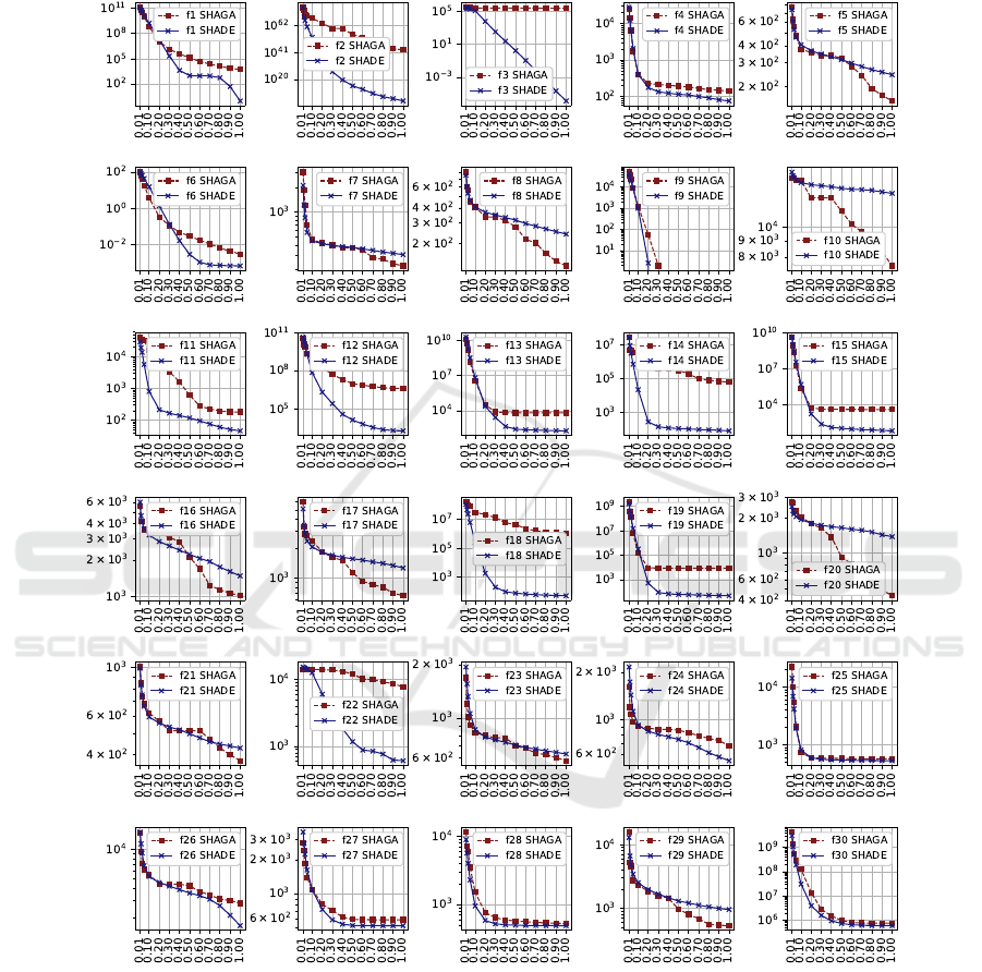
For comparison with other approach the popular
differential evolution algorithm, SHADE, was cho-
sen, as it is known to be one of the most compete-
tive versions of DE according to (Al-Dabbagh et al.,
2018). The same set of CEC 2017 functions was used,
and SHADE had the following parameters: popula-
tion size 75D
2
3
, p parameter in current-to-pbest strat-
egy equal to 0.17, and no archiveset. Table 4 contains
the results of statistical test comparison of SHADE
and SHAGA-c for all functions and all dimensions.
Although the SHAGA-c algorithm is worse than
SHADE in most cases, according to Table 4, one
may observe that SHAGA demonstrates superior per-
formance on several functions for all or most dimen-
sions, including F5, F7, F8, F10, F16, F17, F20,
F23 and F29. Functions F5, F7 and F8 are variants
of Rastrigin function, F10 is Shwefel function, F16,
F17 and F20 are hybrid functions, which also use the
mentioned basic functions, F23 and F29 are composi-
tion functions, also containing Rastrigin and Shwefel
functions. From this, we may conclude that SHAGA-
c is capable of solving problems with many local op-
tima more efficiently then SHADE.
The main reasons of SHAGA high efficiency are
the usage of the specific algorithm scheme, where ev-
ery individual has the possibility to crossover with a
selected individual. Another reason of SHAGA high
quality results is the usage of the parameter tuning
scheme, where the probability of selection and muta-
tion are numerical parameters, but not fixed parame-
Table 4: Statistical test results for SHADE and SHAGA-c.
Func D=10 D=30 D=50 D=100
f1 -1 -1 -1 -1
f2 -1 -1 -1 -1
f3 -1 -1 -1 -1
f4 -1 -1 -1 1
f5 1 1 1 1
f6 -1 -1 -1 1
f7 1 1 1 -1
f8 1 1 1 -1
f9 0 0 0 0
f10 1 1 1 1
f11 1 -1 -1 -1
f12 -1 -1 -1 -1
f13 -1 -1 -1 -1
f14 -1 -1 -1 -1
f15 -1 -1 -1 -1
f16 1 1 1 -1
f17 1 1 1 -1
f18 -1 -1 -1 -1
f19 -1 -1 -1 -1
f20 0 1 1 -1
f21 -1 1 1 -1
f22 0 -1 -1 1
f23 1 1 1 -1
f24 -1 -1 -1 -1
f25 -1 -1 -1 -1
f26 -1 1 -1 -1
f27 -1 -1 -1 -1
f28 -1 -1 -1 -1
f29 1 1 1 1
f30 -1 -1 -1 -1
ter values, as in SelfCGA, where only three mutation
levels are available, and three crossover types.
5 CONCLUSIONS
In this paper the success history adaptation mecha-
nism was applied to the genetic algorithm with a mod-
ified scheme. The newly developed SHAGA algo-
rithm inherited the main loop organization from pop-
ular differential evolution algorithms, such as JADE
and SHADE. In the binary version of SHAGA al-
gorithm two parameters were tuned: the crossover
rate, i.e. the rate of new genetic information, that
will be taken from another individual, and the mu-
tation rate. In the continous version SHAGA-c, the
crossover and mutation distribution indexes were also
tuned. The tuning mechanism was taken from the
mentioned SHADE implementation.
The performed experiments have shown the supe-
rior performance of SHAGA even without parame-
Genetic Algorithm with Success History based Parameter Adaptation
185

ter tuning against another self-tuning meta-heuristic,
SelfCGA on classical binary optimization problems.
With parameter tuning SHA scheme, the results ap-
peared to be even better. Also, it should be noted
that SHAGA used only one selection mechanism,
namely tournament selection with t = 2, while Self-
CGA could automatically choose one of three selec-
tion types. Moreover, for SHAGA, there was only
one crossover type used, i.e. uniform crossover. Ac-
cording to some recent research (Piotrowski and Na-
piorkowski, 2018), many heuristic methods are over-
complicated, and could be significantly simplified,
and SHAGA, even with fixed parameters, demon-
strates the same idea. For binary-encoded numeri-
cal optimization problems SHAGA has outperformed
SelfCGA for most problems in all dimensions. The
presented results have demonstrated that SHAGA not
only gets better result at the end of the search, but also
avoids stagnation.
In comparison with differential evolution based
SHADE algorithm SHAGA has shown superior per-
formance on a number of test functions, which means
that SHAGA’s properties are important for solving
numerical problems with many local optima. As a
result, it could be stated that the newly developed
SHAGA algorithm could be used as a highly com-
petetive genetic algorithm implementation for vari-
ous binary and continous optimization problems, as
well as other problems. The directions of further re-
search may include adding different selective pres-
sure mechanisms for SHAGA, improving the param-
eter tuning scheme, application of external archive or
adding population size adjustment mechanism, such
as linear population size reduction.
ACKNOWLEDGEMENTS
Research is performed with the support of the
Ministry of Education and Science of the Rus-
sian Federation within State Assignment [project #
2.1680.2017/(project part), 2017].
REFERENCES
Al-Dabbagh, R. D., Neri, F., Idris, N., and Baba, M. S.
(2018). Algorithmic design issues in adaptive differ-
ential evolution schemes: Review and taxonomy. In
Swarm and Evolutionary Computation 43, pp. 284–
311.
Deb, K. and Agrawal, R. B. (1995). Simulated binary
crossover for continuous search space. In Complex
Systems, 9(2), pp.115–148.
Deb, K. and Deb, D. (2014). Analysing mutation schemes
for real-parameter genetic algorithms. In Interna-
tional Journal of Artificial Intelligence and Soft Com-
puting 4(1), pp. 1–28.
Eiben, A. E., Hinterding, R., and Michalewicz, Z.
(1999). Parameter control in evolutionary algo-
rithms. IEEE Transactions on Evolutionary Compu-
tation, 3(2):124–141.
Goldberg, D. E. and Deb, K. (1991). A comparative analysis
of selection schemes used in genetic algorithms. In
Vol. 1 of Foundations of Genetic Algorithms, pp. 69–
93. Elsevier.
Piotrowski, A. P. and Napiorkowski, J. J. (2018). Some
metaheuristics should be simpli
ed. In Inf. Sci. 427, pp. 32–62.
Semenkin, E. and Semenkina, M. (2012a). Self-configuring
genetic algorithm with modified uniform crossover
operator. In Advances in Swarm Intelligence. ICSI
2012. Lecture Notes in Computer Science, vol 7331.
Springer, Berlin, Heidelberg.
Semenkin, E. and Semenkina, M. (2012b). Spacecrafts’
control systems effective variants choice with self-
configuring genetic algorithm. In Proceedings of the
9th International Conference on Informatics in Con-
trol, Automation and Robotics, pp. 84–93.
Stanovov, V., Akhmedova, S., and Semenkin, E. (2018). Se-
lective pressure strategy in differential evolution: Ex-
ploitation improvement in solving global optimization
problems. Swarm and Evolutionary Computation.
Tanabe, R. and Fukunaga, A. (2013). Success-history
based parameter adaptation for differential evolution.
In IEEE Congress on Evolutionary Computation, pp.
71–78.
Wu, G., R., M., and Suganthan, P. N. (2016). Problem def-
initions and evaluation criteria for the cec 2017 com-
petition and special session on constrained single ob-
jective real-parameter optimization. In Tech. rep.
Zhang, J. and Sanderson, A. C. (2009). Jade: Adaptive
differential evolution with optional external archive.
In IEEE Transactions on Evolutionary Computation
13, pp. 945–958.
ECTA 2019 - 11th International Conference on Evolutionary Computation Theory and Applications
186
APPENDIX
Figure 3: Convergence of SHAGA and SHADE, D=50.
Genetic Algorithm with Success History based Parameter Adaptation
187
