
Multi-Objective Optimization for Automated Business Process Discovery
Mohamed A. Ghazal
a
, Samy Ghoniemy
b
and Mostafa A. Salama
c
Department of Computer Science, The British University in Egypt, Cairo, Egypt
Keywords:
Multi-Objective Optimization, Process Mining, Multi-Objective Evolutionary Algorithms, Process Model
Discovery, Non-dominated Sorting Genetic Algorithm II.
Abstract:
Process Mining is a research field that aims to develop new techniques to discover, monitor and improve real
processes by extracting knowledge from event logs. This relatively young research discipline has evidenced
efficacy in various applications, especially in application domains where a dynamic behavior needs to be
related to process models. Process Model Discovery is presumably the most important task in Process Mining
since the discovered models can be used as an objective starting points for any further process analysis to be
conducted. There are various quality dimensions the model should consider during discovery such as Replay-
Fitness, Precision, Generalization, and Simplicity. It becomes evident that Process Model Discovery, with its
current given settings, is a Multi-Objective Optimization Problem. However, most existing techniques does
not approach the problem as a Multi-Objective Optimization Problem. Therefore, in this work we propose
the use of one of the most robust and widely used Multi-Objective Optimizers in Process Model Discovery,
the NSGA-II algorithm. Experimental results on a real life event log shows that the proposed technique
outperforms existing techniques in various aspects. Also this work tries to establish a benchmarking system
for comparing results of Multi-Objective Optimization based Process Model Discovery techniques.
1 INTRODUCTION
In the last decade Process Mining has proved its effec-
tiveness in every industrial application and is gaining
popularity among the research community (van der
Aalst et al., 2007). Process mining can be defined
as this emerging discipline providing comprehensive
sets of tools to provide fact-based insights and to sup-
port operational processes. Process model discov-
ery is one of the three main types of process mining
(van der Aalst, 2011) and it is also sometimes referred
to as Workflow Mining (van der Aalst et al., 2004). In
this work (ABPD) will be used which stands for Au-
tomated Business Process Discovery. ABPD aims to
automatically infer process models that accurately de-
scribe any process under analysis by considering only
available records of this process. In other words there
is no prior process model, the model is discovered
based on event logs only.
ABPD is a very challenging task. Naturally event
logs are often noisy, and far from being complete.
(van der Aalst et al., 2004; Van der Aalst et al., 2005).
a
https://orcid.org/0000-0001-5438-9320
b
https://orcid.org/0000-0001-7327-4983
c
https://orcid.org/0000-0003-2559-8056
Adding to this, the quality of the automatically dis-
covered process model should be assessed on several
quality dimensions which are actually competing with
each other (van der Aalst, 2011). Generally speaking,
four quality dimensions are often used to measure the
results of ABPD namely Replay Fitness, Precision,
Simplicity and Generalization. Replay Fitness quan-
tifies the extent to which the discovered model can ac-
curately reproduce the recorded behaviour in the log.
Replay Fitness by itself was widely used as the main
measure for the performance of a process discovery
algorithm because it only makes sense to consider
other dimensions if the replay fitness is acceptable.
Precision ensures that the model does not underfit the
event log. In other words a Precision metric quanti-
fies the fraction of the behavior allowed by the model
which is not seen in the event log. Generalization as-
sesses the extent to which the model generalizes the
behavior in the log to avoid overfitting the data at hand
(i.e. the available traces in the event log). Simplicity
measures the complexity of a model and more often
irrespective of the event log.
Recently, several ABPD techniques have been de-
veloped. Discovering process models which can be
graphically represented in different process modelling
Ghazal, M., Ghoniemy, S. and Salama, M.
Multi-Objective Optimization for Automated Business Process Discovery.
DOI: 10.5220/0008072400890104
In Proceedings of the 11th International Joint Conference on Knowledge Discovery, Knowledge Engineering and Knowledge Management (IC3K 2019), pages 89-104
ISBN: 978-989-758-382-7
Copyright
c
2019 by SCITEPRESS – Science and Technology Publications, Lda. All rights reserved
89

notation. The most prominent discovery techniques
can be roughly categorized into two groups based
on the search strategy and the nature of the algo-
rithm used. The first group uses a local search strat-
egy and here will be referred to as the conventional
techniques. It includes ABPD techniques that uses
general algorithmic approach or a frequency based
heuristics approach. These techniques have some
known drawbacks, especially their inability to focus
on more than one or at maximum two quality dimen-
sions at the same time (Buijs et al., 2012b). Also
conventional ABPD typically generates a single pro-
cess model that may not describe the recorded be-
havior effectively (Buijs et al., 2013). The second
group includes ABPD techniques adopting general
search strategies, mainly a meta-heuristic evolution-
ary approach. The majority of these techniques, ex-
cept for a single one proposed in (Buijs et al., 2013)
uses a single-objective meta-heuristic approach. Con-
sequently, not only it has the same problem as for
the conventional techniques in producing a single so-
lution each run. Moreover, it mainly depends on
the weighted sum method(WSM) (Marler and Arora,
2010). Section 3 of this paper discusses the shortcom-
ings expected with the use of the WSM in more de-
tails. What is important to note here is that even those
techniques used a multi-objective meta-heuristic ap-
proach, none of which used any of the well rec-
ognized Multi-Objective Optimization Evolutionary
Algorithms (MOEAs), such as NSGA-II (Kalyan-
moy et al., 2002), SPEA2 (Zitzler et al., 2000), or
the PAES (Knowles and Corne, 2000). In other
words, the ABPD techniques which adopted a multi-
objective meta-heuristic approaches were focusing on
incorporating some ideas from some notable Pareto-
Front(PF) Based multi-objective optimizers such as
the crowding distance selection (Kalyanmoy et al.,
2002). But never truly considered using one of the
recognized MOEAs. Not only this makes the perfor-
mance of such discovery techniques questionable, but
also raises many other questions such as how to eval-
uate and compare the results of such techniques.
The remainder of the paper is structured as fol-
lows. Next, in Section 2 a literature review on ABPD
is presented. In Section 3 a brief review on Multi-
Objective Optimization(MOO) and a discussion on
what benefits MOEAs can bring to ABPD. Section
4 explain the proposed Multi-Objective Evolutionary
Tree Miner(MOETM) and how it has been built to ex-
tend the Evolutionary Tree Miner(ETM) (Buijs et al.,
2012a) by incorporating a new NSGA-II based evolu-
tionary engine. In Section 5, the proposed technique
was experimented with a real-life event log and the
findings are discussed. Section 6 concludes the paper.
2 PROCESS MODEL DISCOVERY
Since the process model is the starting point for most
of the process mining activities ABPD is one of the
most important research topics in process mining.
As mentioned earlier ABPD aims to discover a pro-
cess model that reflects the causal dependencies of
activities observed in an event log. Then present-
ing the model in one of the process modeling no-
tations. Accordingly, ABPD can be conceived as a
search problem (i.e. a search for the most appropri-
ate process model of the search space of candidate
process models). In the last two decades, various
techniques have been developed (e.g. Alpha (van der
Aalst et al., 2004), Heuristic (Weijters et al., 2006),
Fuzzy (G
¨
unther and Van Der Aalst, 2007), Genetic
Miners (Van der Aalst et al., 2005)) producing pro-
cess models in various forms (e.g. Petri nets, BPMN
models, EPCs, YAWL-models). As in (Van der Aalst
et al., 2005) ABPD techniques can be categorized into
two groups based on the search strategy adopted a lo-
cal or global search strategy. Adding to this and from
a chronological point of view these two categories can
be referred to as conventional ABPD techniques and
the more recent meta-heuristics based ABPD tech-
niques.
2.1 Conventional ABPD Techniques
Table 1: Control-flow discovery algorithms based on their
output model type.
Discovery Algorithm Output model type
-Alpha, Alpha++, and Alpha#
algorithms
-Parikh Language-based Region miner
-Region miner
-Tsinghua-alpha algorithm
-Petrify mining
Petri net
-Duplicate Tasks GA
-Genetic algorithm
-Heuristics miner
Heuristic net
-Frequency abstraction miner
-Fuzzy Miner
Fuzzy model
-FSM miner
-k-RI Miner
Finite state machine
/ Transition system
-Multi-phase Macro Plugin EPC Event-driven
Process Chain
-DWS mining plug-in
-Workflow patterns miner
Other
ABPD techniques adopting a local search strat-
egy by means of using a general algorithmic or a
KDIR 2019 - 11th International Conference on Knowledge Discovery and Information Retrieval
90

frequency based heuristics approach here will be re-
ferred to as conventional techniques. Table 1 list
the most notable and widely used of these techniques
based on their output model type. Lack of space al-
lows us only to summarize the literature review re-
garding the conventional techniques. If more back-
ground on this topic is required, there are several good
references that the reader is invited to consult such as
the literature reviews and the comparative studies in
(Gupta, 2014; Tiwari et al., 2008). What could be
said briefly here is that these conventional techniques
are known for the following problems:
• These techniques typically returns a single process
model each run, which sometimes may not be able to
effectively describe the recorded behavior (Buijs et al.,
2013).
• They suffer the inability to focus on more than one or
two quality dimensions at the same time (Buijs et al.,
2012c).
• A major drawback is that they can not mine all the com-
mon constructs of a process model (Van der Aalst et al.,
2005). Such Problematic constructs are discussed in
details in (de Medeiros, 2006).
2.2 Meta-heuristic ABPD
The first time a meta-heuristic method was used in
ABPD was when the authors in (de Medeiros, 2006)
used a Genetic Algorithm (GA) to discover process
models represented in petri-nets. In (de Medeiros,
2006) the author used a two dimensional fitness mea-
sure. There was a problem with the measurement of
the preciseness dimension and it was actually claimed
that it is not practical to accurately measure this di-
mension. Moreover the genetic process model discov-
ery algorithm suffered from the long execution time.
In (Bratosin et al., 2010a), it was argued that the fit-
ness calculation phase of the algorithm was the main
reason for the long running time and a sampling tech-
nique to address the issue was proposed. A sample
of the event log in the fitness calculation phase was
used instead of the whole log. In (Bratosin et al.,
2010b) a distributed architecture for the genetic pro-
cess discovery algorithm was proposed to further im-
prove the performance regarding the execution time.
The work in (Tsai et al., 2010) extended the work in
(de Medeiros, 2006) by adding a time interval analy-
sis between the events. In all of the studies mentioned
so far petri-nets were used as the internal represen-
tation. The use of petri-nets as an internal represen-
tation was a fundamental reason behind the genetic
ABPD limited performance. One of the main require-
ments for an ABPD technique is to produce error-free
models, also known as sound models. A definition for
the notion of soundness for petri-nets can be found in
(van der Aalst et al., 2011), likewise a deep analysis
for all important requirements which should be con-
sidered when choosing a suitable process model no-
tation for a process discovery algorithm can be found
in the PhD dissertation in (Buijs, 2014).
The work in (Buijs et al., 2012b) proposed the use
of a tree representation to ensure the soundness of the
model. Process trees (Buijs, 2014) ensured sound-
ness since block-structured process models are inher-
ently sound because they require that each control-
flow split has a corresponding join of the same type.
An example illustrating the notion of process discov-
ery using process trees can be found in the first sec-
tion (Introduction) in (Buijs et al., 2012b). The use
of process trees as an internal representation in a ge-
netic ABPD not only ensures a sound model in the fi-
nal output. Moreover, it improves the performance of
the genetic algorithm due to the considerable reduc-
tion in the size of the search space. When using Petri-
nets to describe process models, the search space con-
sists of all possible Petri-nets of both correct and in-
correct models. However, process trees regardless of
how they are created, are always sound process mod-
els. This means that many of the unwanted unsound
models are not going to be created in the first place
resulting a reduction in the size of the search space.
In addition to introducing process trees the work in
(Buijs et al., 2012b) also proposed a new fitness mea-
sure reflecting the quality metrics for process models
described in (van der Aalst, 2011).
All previous studies mentioned so far use a clas-
sical optimization method by converting a multi-
objective optimization problem (MOP) into a single-
objective optimization problem (SOP) and empha-
size one particular optimal solution as the final result.
Generating a single process is not the only problem
these techniques suffers. Most importantly these tech-
niques use the weighted sum method to reformulate
the MOP into an SOP. The WSM has some known
drawbacks when used for solving MOPs (Marler and
Arora, 2010). The next section in this paper discusses
this in a bit more details and it will become apparent
that especially in the case of genetic ABPD the WSM
may not be a good choice. To the best of our knowl-
edge only one case study adopts a multi-objective
optimization approach in ABPD. The researchers in
their work in (Buijs et al., 2012b) concluded that of-
ten is not one single process model that describes the
observed behavior best in all quality dimensions. Mo-
tivated by the findings in their previous work they fur-
ther extended it in (Buijs et al., 2013) to obtain a col-
lection of mutually non-dominating process models.
While the proposed algorithm is following a multi-
objective optimization methodology and even uses
Multi-Objective Optimization for Automated Business Process Discovery
91

a fitness function inspired by the crowding distance
used in NSGA-II. However, there are some funda-
mental differences between the solution proposed in
(Buijs et al., 2013) and most of the recognized Multi-
Objective Evolutionary Algorithms (MOEAs). The
size of the Pareto-Front which is unbounded by any
limits such as the size of the population, the overall
fitness calculation, and the selection strategy are some
of these notable differences. Hence, from a MOO
point of view the performance of this solution remains
questionable. In addition, how to assess the perfor-
mance of MOO techniques in the context of ABPD
and how to compare its outcomes represent a far more
interesting research questions.
3 MULTI-OBJECTIVE
OPTIMIZATION
Optimization refers to find the best possible solu-
tion to a problem given a set of limitations (or con-
straints). When building an optimizer for a SOP, the
aim is to find the best possible solution available (i.e.
global optimum) or at least a good approximation of
it. However, in most real world problems there is
not one but several objectives to be optimized simul-
taneously. And in fact it is normally the case that
these objectives are in conflict with each other. These
problems with two or more objective functions are
called MOPs and require different mathematical and
algorithmic tools than those adopted to solve SOPs
(Tamaki et al., 1996). Moreover, even the notion
of optimality changes when dealing with MOPs. In
MOP the optimization result is not a single solution
like in SOP rather its a set of solutions. And it is of-
ten unclear which one constitutes an optimal solution.
A solution may be optimal for one objective function
but sub-optimal for another. Thus, it is required to
find a number of solutions in order to provide the de-
cision maker with insight into the characteristics of
the problem before a final solution is chosen (Marler
and Arora, 2004). The set of solutions, which are the
optimization result of an MOP are often called Pareto-
Front (PF). The basic idea is to obtain a set of solu-
tions which are mutually non-dominating. A solution
dominates another if for all objective functions it is at
least equal or better, and is strictly better in at least
one objective.
3.1 The Weighted Sum Method (WSM)
The main goal in solving a MOP is to obtain a Pareto-
optimal set (or to sample solutions from the set as
uniformly as possible). Classical optimization meth-
ods suggest converting the MOP into a SOP by em-
phasizing one particular Pareto-optimal solution at a
time (Kalyanmoy et al., 2002). When there is a need
to find multiple solutions using this method it has
to be applied many times hopefully finding a differ-
ent solution at each simulation run. Several methods
were proposed to convert a MOP into an appropri-
ately formulated SOP. Despite deficiencies with re-
spect to depicting the Pareto-optimal set the WSM
continues to be used extensively in MOO (Marler and
Arora, 2010). And in the case of ABPD there is no
much difference as it is observable that all discov-
ery techniques which employed a meta-heuristic ap-
proach (de Medeiros, 2006; Bratosin et al., 2010a;
Bratosin et al., 2010b; Tsai et al., 2010; Buijs et al.,
2012a) except for (Buijs et al., 2013), used the WSM.
However, this method is known for its weaknesses in
solving MOPs. According to (Buijs et al., 2013) the
following drawbacks can be listed:
• Determining the correct weights upfront is difficult. A
small change in in weights may results in big changes
in the objective vectors.
• Since only one solution is returned if the solution is not
acceptable due to inappropriate setting of the weights,
new runs of the optimizer is required
More importantly the following should also be em-
phasize. Generally speaking, the WSM is having a
widely known problem of being very sensitive to the
shape of the Pareto frontier (convex, or concave) or
to discontinuous Pareto fronts. In (Marler and Arora,
2010) it is stated that many case studies demonstrated
the method’s inability to capture Pareto optimal points
that lie on non-convex portions of the Pareto optimal
curve. It is also acknowledged the method does not
provide an even distribution of points in the Pareto
optimal set. This will have a crucial impact in the
case of ABPD. ABPD is currently being solved as
a maximization MOP and with its current settings a
non-convex if not a concave shape of the PF is often
expected. Figure 1 illustrates the expected shape of
the PF in both minimization and maximization prob-
lems along with ideal and nadir points in both cases.
More resources and information on the WSM and the
notion of convexity (concavity) is in Appendix B.
3.2 Multi-Objective Evolutionary
Algorithms (MOEAs)
One of the most successful methods applied to ob-
tain a PF in MOO is evolutionary algorithms (EAs).
The main reason for this is their ability to find mul-
tiple Pareto optimal solutions in one single simula-
tion run (Kalyanmoy et al., 2002). In the last two
KDIR 2019 - 11th International Conference on Knowledge Discovery and Information Retrieval
92

Figure 1: Pareto front with ideal and nadir points for mini-
mization and maximization problems, from (Ishibuchi et al.,
2017).
decades a number of MOEAs have been suggested.
The most prominent are NSGA-II (Kalyanmoy et al.,
2002), PAES (Knowles and Corne, 2000), and SPEA-
II) (Zitzler et al., 2000). Several studies had exten-
sively compared them and other MOEAs regarding
their performance, but no clear overall winner can
be announced (Gadhvi et al., 2016). MOEAs perfor-
mance assessment in and of itself is a very active re-
search area. In fact the amount of effort in this area of
research is immense and several innovations in vari-
ous studies can be found (e.g. (Knowles et al., 2006;
Azarm and Wu, 2001; Li et al., 2014; Schott, 1995;
Van Veldhuizen, 1999; Riquelme-Granada et al.,
2015)). However, the lack of a unified MOEA Evalua-
tion Framework to systematically compare algorithms
which can be used and extended by researchers to
benchmark the different algorithms makes compar-
ing the different algorithms a bit problematic. As de-
scribed in (Riquelme-Granada et al., 2015), a MOEA
main goal it to both converge close to the real, yet un-
known, PF and at the same time maintain a good di-
versity among the solutions on the current PF. There-
fore, the research efforts focuses on developing vari-
ous Quality Indicators (QIs) to evaluate the MOEA
Convergence and Diversity. Convergence metrics are
concerned with ensuring whether the non-dominated
solutions in the obtained PF is close to the true op-
timal Pareto Front(PF
t
) and whether it covers the
whole extension of the PF
t
. Notice that when the PF
t
is unknown a reference set is considered instead. Di-
versity metrics are to indicate whether the obtained
solutions are well spread and spaced among each oth-
ers. In other words Diversity evaluates both the uni-
formity and spread. Uniformity and spread are two
very closely related facets, yet they are not completely
the same (Riquelme-Granada et al., 2015). Accord-
ingly, the Quality Indicators can be classified based
on the aspect that a QI measures as follows:
• Convergence metrics: Indicates how distant an approxi-
mation set from the true Pareto optimal front (e.g. Gen-
erational distance (GD) (Van Veldhuizen, 1999), Dom-
inance Ranking (Knowles et al., 2006)).
• Cardinality metrics: The number of solutions that ex-
ists in the obtained Pareto Front. Intuitively, a larger
number of solutions is preferred (e.g. Generational
Nondominated Vector Generation (GNVG) (Van Veld-
huizen, 1999)).
• Uniformity metrics: The distribution, refers to the rela-
tive distance among solutions in Pareto Front(e.g. Spac-
ing (Schott, 1995)).
• Spread metrics: Also known as the extent, refers to the
range of values covered by the solutions (e.g. Overall
Pareto Spread (Azarm and Wu, 2001)).
In this study a single QI was chosen from each of the
previously illustrated categories based on a criterion
presented in section 5 of this paper. Also the criteria
used for choosing which MOEA to be implement in
the proposed solution is presented in the next section.
4 MULTI-OBJECTIVE
EVOLUTIONARY TREE MINER
ProM framework (Verbeek et al., 2010) is the de
facto standard process mining platform in the aca-
demic world. In fact most of the previously men-
tioned ABPD techniques were implemented as plug-
ins for the ProM framework. The work in (Buijs
et al., 2012a) has been implemented as a plug-in for
the ProM framework, namely the Evolutionary Tree
Miner (ETM). Also, the work in (Buijs et al., 2013)
has been implemented as the ETM with the Pareto-
Front extension (ETM-Preto used in the following).
Since the ETM is an extensible evolutionary pro-
cess discovery algorithm it was decided to extend the
ETM in the solution proposed in this paper. Not only
this will save a considerable amount of time and re-
sources, but also it enables conducting a more objec-
tive comparison when ones considers comparing the
performance of the solution proposed in this paper to
the previously proposed solutions such as the one in
(Buijs et al., 2013). Initially, it was decided to choose
the MOEA to be implemented based on the simple
criteria:
• The algorithm must support elitism.
• The algorithm should be a parameter-less GA, i.e. there
is no need to specify any parameters (e.g. niching oper-
ators).
• The algorithm is simple and straightforward.
• Relatively fast, with an overall complexity of O(MN
2
) or
better.
• Converges steadily and fast towards Pareto front.
However, since NSGA-II meets all of the require-
ments above, and since the solution proposed in
(Buijs et al., 2013) is using a fitness calculation in-
spired by the crowding distance used in the NSGA-
II. Again, in order to include greater objectivity in
Multi-Objective Optimization for Automated Business Process Discovery
93
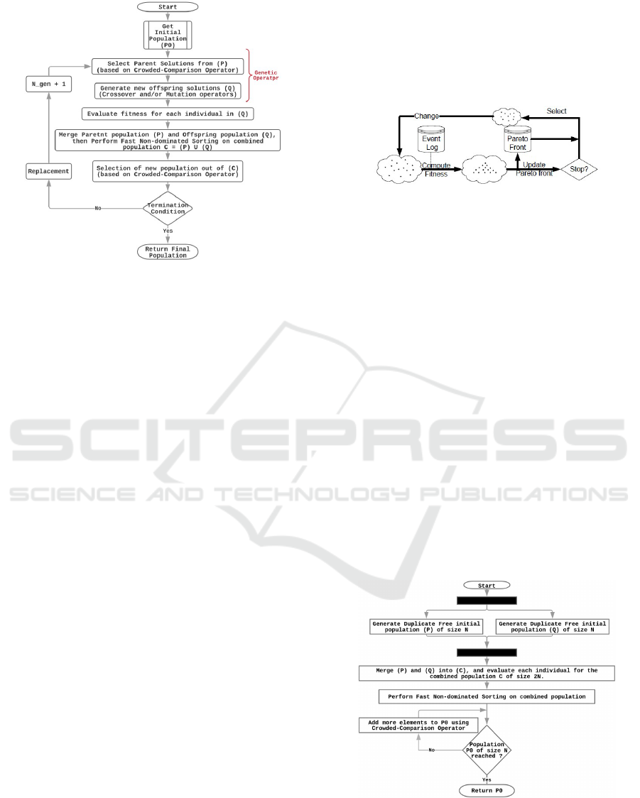
Figure 2: MOETM / NSGA-II based ABPD.
the correlation, the decision was made to implement
NSGA-II.
The ABPD technique proposed in this paper has
been implemented as a ProM plug-in namely Multi-
Objective Evolutionary Tree Miner (MOETM). Fig-
ures 2 and 3 depicts how both algorithms MOETM,
and ETM-Pareto works respectively. For a de-
tailed description of how the ETM-Pareto works,
please review (Buijs et al., 2013) (section 3). The
MOETM implements the NSGA-II originally pro-
posed in (Kalyanmoy et al., 2002) with a slight differ-
ence in the first step of the algorithm Generating Ini-
tial Population. Evaluating MOETM initial results, it
was observed that duplicates are negatively affecting
the performance of the algorithm in a way that can-
not be overlooked. In order to reduce the impact of
duplicates from the beginning and to improve diver-
sity in the initial population the procedure Get Initial
Population, depicted in Figure 4, was introduced. In
NSGA-II there are two kinds of populations P
t
and Q
t
.
Assuming that population size is referred to as N and
Generation number as N
Gen
. Originally in NSGA-II
creating the initial population is as follows: A random
parent population P
t
of size N is created. The popula-
tion is sorted based on the non-domination then each
solution is assigned a fitness (or rank) equal to its non-
domination level (1 is the best level, 2 is the next-best
level, and so on). Thus, minimization of fitness is
assumed. At first, the usual binary tournament selec-
tion, recombination, and mutation operators are used
to create an offspring population Q
t
size N. While
Generating Initial Population in MOETM is as fol-
lows: When N
G
en = 0, initialize both initial P and
initial Q randomly using a duplicate eliminator pro-
cedure. Combine both P and P in C and calculate the
different quality dimensions for each candidate in C.
Perform Fast-non-dominated sorting, and if necessary
crowding distance selection on C to get P
t
of size N.
Rest of the Procedures in MOETM are identical to
the original NSGA-II. Detailed description for rest of
procedures in NSGA-II can be found in (Kalyanmoy
et al., 2002) (section 3).
Figure 3: The different phases of the ETM-Pareto genetic
algorithm (Buijs et al., 2013).
Both ETM-Pareto and MOETM envision the same
approach to solve the problem of process model dis-
covery, both algorithms deal with ABPD as a MOP
and are trying to obtain an approximation set as close
as possible to the (PF
t
). However, there are some fun-
damental differences in how each algorithm works.
Especially, in the way the PF is constructed and main-
tained internally in each algorithm. In ETM-Pareto,
the PF represents an autonomous construct somehow
independent from the current population in every gen-
eration. It was expected that this implementation with
the unlimited size PF, which is unbounded by any
limits such as the size of the population, will have its
impact on the performance of the ETM-Pareto. While
this unlimited size Pareto-Front allows for the oppor-
tunity to guarantee inclusion of optimal solutions in
each generation. However, the simulation results and
analysis in the next section will demonstrate that this
approach has a negative impact on the overall perfor-
mance of the ETM-Pareto algorithm as expected.
Figure 4: MOETM Get-Initial-Population Procedure.
KDIR 2019 - 11th International Conference on Knowledge Discovery and Information Retrieval
94

5 SIMULATION AND RESULTS
In the following subsections, we first describe the en-
vironment in which the experiment was conducted,
the used data set, the experiment parameters values,
and the platform. The quality indicators used to as-
sess the performance of the two algorithms are pro-
vided in the next subsection, followed by a detailed
description of the comparative results.
5.1 Testing Environment
The data set is a real-life event log from Volvo
IT Belgium which was available for the Third In-
ternational Business Process Intelligence Challenge
(BPIC’13) (Verbeek, 2016). The log contains events
from an incident and problem management system
called VINST. More information about the data set
as well as documents detailing the data set is avail-
able in (Verbeek, 2016). The third log file (The prob-
lem management log-closed problems) was chosen as
a start to test the proposed technique. The event log
contains 1487 traces and 6660 events in total.Since
the study focuses on the benefits of using NSGA-II in
ABPD, and since this is the first time a well tested and
proven MOEA is applied in ABPD therefore ETM-
Pareto results will be used as the control group. All
parameters in both groups were kept the same such
as the style and the rate of crossover and mutation.
The probability of performing crossover and muta-
tion was 0.1 and 0.5 respectively. Both algorithms
ran for 50 times. A maximum generations number
of 300 and a total population size of 100 were used.
Any differences in the settings were mainly due to the
different nature of the two algorithms. For instance,
ETM-Pareto was assigned an elite count of size 20.
On the other hand the MOETM does not require any
parameters such as elite size since elitism in NSGA-
II works differently. Finally, for the selection strat-
egy the MOETM used the tournament selection while
ETM-Pareto was left with its default settings using
Sigma Scaling. The experiment was performed on a
machine running Windows 10 64-bit with 4 cores In-
tel Core i7-4710HQ Processor running at 2.50 Ghz
and 8 GB memory, of which maximum of 5 GB was
used by the algorithms.
5.2 Quality Indicators
As discussed earlier, in MOO two aspects should be
considered and both should be measured simultane-
ously. First, to what extent the obtained solutions
converge to the PF
t
. Secondly, to what extent these
solutions are distributed. In Section 3 of this paper it
was discussed how the most prominent QIs can be cat-
egorized where a grouping as in (Riquelme-Granada
et al., 2015; Li et al., 2014) was followed. Due to
the large number of QIs available, also these metrics
ranges from straightforward and easy to compute to
the not so easy and computationally intensive. The
following criteria were developed to choose a single
QI from each category:
• Reliability, the QI has been used frequently in recent
case studies, and its usage reflects an unfaltering qual-
ity.
• The QI should be straightforward and computationally
inexpensive.
• The QI does not require prior knowledge of the PF
t
.
• The QI does not use reference sets or reference points.
Based on the criteria defined above, the following QIs
were being chosen to evaluate the performance.
5.2.1 QI for Evaluating
Convergence / Outperformance
Generally, there are various types of accuracy QIs de-
pending on whether the PF
t
is known or not. When
the PF
t
for a given problem is known accuracy QIs
usually focuses on quantifying the rate of how many
real PF
t
solutions exist among all non-dominated so-
lutions
1
returned by the MOEA, or the distance how
far the non-dominated solutions are from the PF
t
.
When the PF
t
is unknown accuracy QIs usually uses
a reference point or a reference set instead. Since
the PF
t
for a process model discovery problem is un-
known and since it was decided not to use any QI that
depend on a reference point the Dominance Ranking
introduced in (Knowles et al., 2006) is used. Dom-
inance Ranking compares the quality of PFs gen-
erated by two or more MOEAs. It is a binary or
even arbitrary QI (i.e., it takes as an input two or
more PF results of two or more MOEAs). Dom-
inance Ranking has the following definition. Sup-
pose q ≥ 2 is the number of MOEAs to be com-
pared. For each MOEA i ∈ {1, . . . , q}, a number of
runs r
i
≥ 1 are performed, generating approximation
sets A
1
1
, A
1
2
, . . . , A
1
r
1
, . . . , A
q
1
, . . . , A
q
r
q
, and C is the com-
bined collection of all approximation sets. Each ap-
proximation set in C is assigned a rank, on the basis
of dominance relations listed in Table 2 in (Knowles
et al., 2006), by counting the number of sets by which
a specific approximation set is dominated.
rank(C
i
) = 1 + |{C
j
∈ C : C
j
CC
i
}|.
(1)
The lower the rank, the better the corresponding ap-
proximation set with respect to the entire collection.
1
Solutions returned by a stochastic multiobjective optimizer
are known as the PF, approximation set, or non-dominated
set (NDS).
Multi-Objective Optimization for Automated Business Process Discovery
95

5.2.2 Cardinality QI
For an approximation set A as a result of multi-
objective optimizer, the cardinality of A refers to the
number of solutions that exists in A. Intuitively, a
larger number of solutions is preferred.
Generational Nondominated Vector Generation
(GNVG) is a simple metric that tracks the number
of non-dominated vectors produced each MOEA gen-
eration. GNVG was introduced in (Van Veldhuizen,
1999) and is defined in equation 2.
GNV G , |PF
current
(t)|
(2)
5.2.3 Spread QI
The primary goal for a multi-objective optimizer is
to provide the decision maker with a large enough
but limited number of solutions. Also it is highly de-
sirable that this limited number of solutions are uni-
formly spread over the whole PF and are as diverse as
possible. The QIs under Pareto spread are concerned
with the range of objective function values. An ap-
proximation set that spreads over a wider range of the
objective function values provides the designer with
broader optimized design choices. In (Azarm and
Wu, 2001) the researchers introduced a spread metric
that quantifies how widely the obtained approxima-
tion set spreads over the objective space when the ob-
jective functions are considered altogether. The Over-
all Pareto Spread (OS) is defined as the volume ra-
tio of two hyper-rectangles. One of these rectangles
is HR
gb
that is defined by the good and bad points
with respect to each design objective. Similarly, the
extreme points for an observed Pareto solution set
defines the other hyper-rectangle that is denoted by
HR
ex
. The overall Pareto spread is defined as the ra-
tio of the area or volume of HR
ex
to that of HR
gb
:
OS(P) =
HR
ex
(P)
HR
gb
(3)
where P refers to an observed approximation set. By
using the objective values to interpret HR
ex
(P) and
HR
gb
, equation 3 can be expressed as:
OS(P) =
m
∏
i=1
|max
np
k=1
(P
k
)
i
− min
np
k=1
(P
k
)
i
m
∏
i=1
|(P
b
)
i
− (P
g
)
i
|
=
m
∏
i=1
|max
np
k=1
[ f
i
(x
k
)] − min
np
k=1
[ f
i
(x
k
)]|
(4)
5.2.4 Uniformity QI
A Spread QI alone will not be able to fully charac-
terize the diversity of solutions in a given approxima-
tion set. If the solutions in a given approximation set
are all very similar, these solutions will not be able
to reflect the trade-offs between the different objec-
tives. Uniformity QI measure the evenness of dis-
tribution of solutions across the PF. A measure of
uniform distribution (UD) to measure the distribution
of non-dominated individuals was proposed in (Tan
et al., 2002) . Mathematically, UD(X
0
) for a given set
of non-dominated individuals X
0
in a population X,
where X
0
⊆ X , is defined as
UD(X
0
) =
1
1 + S
nc
(5)
where S
nc
is the standard deviation of niche count of
the overall set of non-dominated individuals formu-
lated as,
S
nc
=
v
u
u
u
u
t
N
x
0
∑
i
nc(x
0
i
) − nc(X
0
)
N
x
0
− 1
(6)
where N
x
0
is the size of the set X
0
, nc(x
0
i
) is the niche
count of i
th
individual x
0
i
where x
0
i
∈ X
0
, and nc(X
0
) is
the mean value of nc(x
0
i
), ∀ i = 1, 2, . . . , N
x
0
as shown
in the following equations:
nc(x
0
i
) =
N
x
0
∑
j, j6=i
f (i, j),
where f (i, j) =
1, dis(i, j) < σ
share
0, else
(7a)
(7b)
nc(X
0
) =
N
x
0
∑
i
nc(x
0
i
)
N
x
0
(8)
where dis(i, j) the distance between individual i and
j in the objective domain. In the paper, σ was set to
0.01. Generally speaking, the larger the spread the
better it is, as it means a better distribution.
5.3 Result Analysis
A real-life event log was used to test and verify the
validity of the newly proposed MOEA based ABPD
technique. The ETM-Pareto acts as the control group
and all settings are the same. Four Quality Indicators
of four different types are used to evaluate the validity
of the proposed technique more comprehensively.
Table 2 demonstrates a sample of the obtained re-
sult in a randomly chosen five runs of both engines
(10, 20, 30, 40, and 50). In Table 2 the size of the final
approximation set PF-size and the corresponding UD,
OS values obtained by MOETM and ETM-Pareto are
provided. Along with the first process model (repre-
sented by the scores that model obtains on each qual-
ity dimension) to exist in that final approximation set.
Interestingly, in all the cases, the MOETM attains a
considerable better UD and OS. Even with its PF-size
far less than of the control group. Which indicates
that all approximation sets obtained by the MOETM
KDIR 2019 - 11th International Conference on Knowledge Discovery and Information Retrieval
96
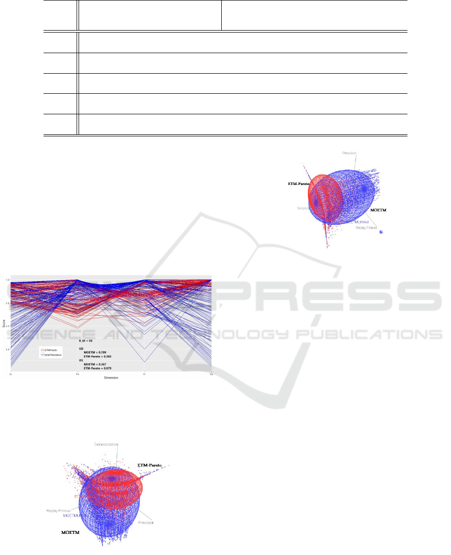
Table 2: A sample of results in a randomly chosen five runs (Run-ID) 10, 20, 30, 40, and 50.
Run-ID Engine-Name UD OS PF-size Sample candidate
Replay-Fitness Precision Simplicity Generalization
10
MOETM 0.741 0.547 100 1 0.801 0.739 0.630
ETM-Pareto 0.313 0.339 194 0.844 0.992 0.916 0.881
20
MOETM 0.730 0.8991 100 1 0.850 0.75 0.683
ETM-Pareto 0.367 0.0718 116 0.827 0.998 0.9 0.869
30
MOETM 0.713 0.515 100 1 0.754 0.972 0.906
ETM-Pareto 0.426 0.264 196 0.733 0.999 0.666 0.647
40
MOETM 0.753 0.481 100 1 0.728 0.928 0.817
ETM-Pareto 0.455 0.174 174 0.988 0.886 0.933 0.900
50
MOETM 0.709 0.367 100 1 0.822 0.937 0.853
ETM-Pareto 0.383 0.079 356 0.800 0.998 0.888 0.847
has a much better distribution and spread over the PF.
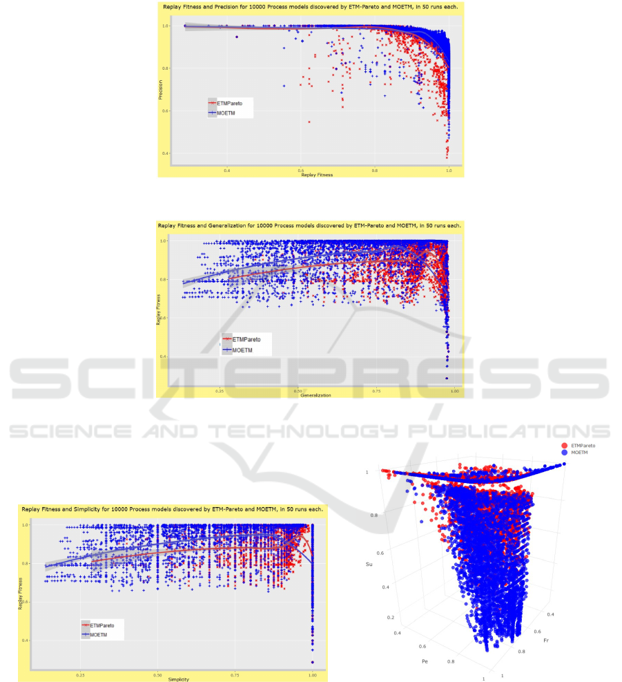
Furthermore, and regarding the quality of the process
models obtained by both engines, as figure 5 illus-
trates it is observable that the models obtained by the
MOETM scores best on the Replay-Fitness(FR) fol-
lowed by Precision(PE) then and at the same time has
an acceptable and a more diverse scores on the other
two quality dimensions Simplicity(SU) and Gener-
alization(GV). More analysis results are available in
Appendix A.
Figure 5: Process models scores on Four quality Dimen-
sions FR, SU, GV, and PE for models obtained by both en-
gines MOETM(Blue) and ETM-Pareto(Red) in the last run
(R-ID = 50) along with UD and OS scores of each engine.
Figure 6: All Approximation Sets obtained by both
MOETM(Blue) and ETM-Pareto(Red) on three dimensions
Replay Fitness, Precision, and Generalization.
Figure 7: All Approximation Sets obtained by both
MOETM(Blue) and ETM-Pareto(Red) on three dimensions
Replay-Fitness, Precision, and Simplicity.
In (Knowles et al., 2006) it is recommended that
the Dominance Ranking is to be used as the first QI.
Since if a significance difference can be demonstrated
using the ranking of approximation sets alone, there
will be no need to use other QIs to conclude which
of the MOEAs generates the better sets. In our case
the Dominance Ranking QI did not reveal much dif-
ference in the ranking of approximation sets proba-
bly due to the large size of the final approximation
sets (100 in case of MOETM and more than 100 in
for ETM-Pareto) along with a relatively low number
of maximum generations (300). A maximum gen-
eration number of 300 may be considered to be low
for such kind of experiment especially with the given
settings. Originally, it was decided that the exper-
iment will have a maximum generation number of
2000. However, the number of generations had to be
reduced due to the inability of ETM-Pareto to finish
execution successfully. Even with a maximum gener-
ation number of 500, ETM-Pareto was unable to suc-
cessfully finish execution for three times. This prob-
lem is an inherent problem for the ETM-Pareto, and
its main reason is the unlimited size of the PF the
ETM-Pareto maintains internally. While this imple-
mentation guarantees that the PF keeps all elite non-
dominated candidates found in all previous genera-
tions. However, Always the moment will come when
the size of the maintained PF exceeds the upper lim-
Multi-Objective Optimization for Automated Business Process Discovery
97
its of the available computational resources. When
that moment comes, the engine will be forced to stop
running. This premature end of execution is depriv-
ing the algorithm the chance of exploring more can-
didates which could be more optimal and can replace
some or maybe many of the existing elite candidates
existing in the PF. No matter how much computa-
tional resource are available (e.g., RAM size avail-
able and allocated), with this implementation it will
never be guaranteed to avoid this problem. And due
to the stochastic nature of MOEAs its could happen
in early or late generations. MOETM does not suf-
fer such problem since the PF size is always trimmed
and is guaranteed to be less than or equal to the size
of the population.
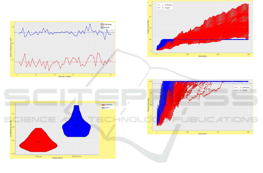
Figure 8: UD in 100 Approximation Sets for both MOETM
and ETM-Pareto (50 Approximation sets each).
Figure 9: OS in 100 Approximation Sets for both MOETM
and ETM-Pareto (50 Approximation sets each).
Since high-dimensional visualization and includ-
ing more than three-dimensions at once is very diffi-
cult and sometimes incomprehensible. Two and three
dimensional plotting will be used to visualize the PF
and the improvements achieved in the quality of the
obtained PF represented in a better spread and uni-
formity. Figure 7, and figure 6 shows a distribu-
tion of Approximation Sets (NDSs) obtained by both
MOETM, and ETM-Pareto on three different process
model quality dimensions. It is visually observable
that in both figures the MOETM has a larger and an
even spread of solutions. Figure 8 shows the UD of
every PF obtained in each of the runs for both algo-
rithms. The figure shows that in all of the 50 runs
the MOETM has a better UD. The MOETM has a
minimum UD of 0.65 while the maximum U D for
ETM-Pareto was 0.48. Overall, the MOETM has an
average UD of 0.733 while the control group has an
average UD of 0.372. Similarly, figure 9 shows that
the MOETM has minimum and maximum OS of 0.32
and 0.91 respectively while ETM-Pareto has a maxi-
mum OS of 0.48 and a minimum OS of 0.03. Overall,
the MOETM has an average OS of 0.523 while the
control group has an average OS of 0.214. Although
the ETM-Pareto usually has a larger PF size than it of
MOETM. However, the MOETM maintained a much
better diversity in the obtained solutions in all runs.
Figure 10: GNVG in 100 Approximation Sets for both
MOETM and ETM-Pareto in all 300 Generations.
Figure 11: GNVG in 100 Approximation Sets for both
MOETM and ETM-Pareto in all 300 Generations, imited
to maximum Approximation Set size of 100.
From a point of view considering cardinality QIs,
it is true that an optimizer which can obtain a larger
PF size is preferred. And it is also true that the ETM-
Pareto always returned a PF of a larger size than
MOETM. However, we believe this measure is mis-
leading in our case. First, early it was explained that
the untrimmed PF of ETM-Pareto is the reason be-
hind its larger PF size, also it was demonstrated ear-
lier what side effects this has on the overall perfor-
mance of the algorithm. Second, the GNVG QI indi-
cates that the MOETM has a faster convergence and
always obtained a larger Approximation set earlier
than the control group. Figure 10 shows the GNVG
for both algorithms in all 300 generations (all Ap-
proximation sets included). Figure 11 is basically a
zoom-in version of figure 10 where the Y axis (the
axis representing the Approximation set size) is lim-
ited to 100 (the maximum size of population). As
KDIR 2019 - 11th International Conference on Knowledge Discovery and Information Retrieval
98

figure 11 shows it was observed that in all runs the
MOETM was faster in getting a non-dominated set
of solutions with larger size (e.g., the ETM-Pareto
has never reached a non-dominated set of solutions
with size of 100 before the 50th generation, while
MOETM had this size in some runs before the 25th
generation).
6 DISCUSSION, CONCLUSIONS
AND FUTURE WORK
In this paper a Multi-Objective Optimization based
Process Model Discovery technique is presented. The
proposed solution has been implemented as a plug-in
for the ProM framework named the Multi-Objective
Evolutionary Tree Miner (MOETM). The MOETM is
an extension to the infamous Evolutionary Tree Miner
(ETM) with a new evolutionary engine based on the
NSGAII. The proposed ABPD technique is able to
obtain a Pareto Front of mutually non-dominating
process models. The MOETM was tested on a real-
life event log and the results were compared to a con-
trol group of the ETM-Pareto. In order to systemat-
ically and accurately compare the results of the two
algorithms, four different Quality Indicators were im-
plemented to assess the quality of both convergence
and diversity in the final approximation set.
The results shows that the MOETM had a faster
convergence toward the Pareto front. Results also
demonstrated that the MOETM had a vastly improved
distribution characteristic evident in the much bet-
ter spread and uniformity of its obtained results. In
comparison to the control group, the MOETM av-
erage Uniform Distribution was better by 97.04% ,
and it had a 144.39% increase in the average Overall
Pareto Spread. This paper also points out the poten-
tial problem the original ETM may suffer. The ETM
will more likely return sub-optimal or extremal so-
lutions (Emmerich and Deutz, 2018) due to the use
of the weighted sum method. The experiment shows
that ETM-Pareto sometimes had improper termina-
tion due to its Pareto Front of unlimited size. It is
clear that truncation of the Pareto Front and keeping
its size under a certain limit is necessary in stochas-
tic multi-objective optimizers to avoid running out of
computational resources in late generations and to en-
sure proper termination. Moreover, and also from a
stand point considering MOO, there exists plenty of
MOEAs Frameworks available (e.g. Opt4J, MOEA,
ECJ, and JMetal (Durillo and Nebro, 2011)) but there
is a need for a MOO Framework with a non-invasive
API like the Watchmaker Framework (Dyer, 2010)
which currently supports only SOO. Such a frame-
work with a non invasive API will allow researchers
to put to the test different MOEAs to solve vari-
ous problems in many application domains with more
ease.
Future work will focus on investigating the use of
other MOEAs in ABPD and the inclusion of other
QIs to assess the results of MOEAs in the context
of ABPD. Especially, convergence QIs as there is a
need for a more accurate but at the same time less
computationally expensive metrics to assess the con-
vergence in MOEAs. Furthermore, MOEAs returns
a Pareto Front as its final output. This Pareto Front
is a set of mutually non-dominated optimal solutions.
Since, this set is usually very large and the decision
maker faces the problem of reducing the size of this
set to a manageable number of solutions to analyze.
There is a need for investigating an approach which
can objectively reduces the non-dominated set of so-
lutions obtained by a MOEA, or even better, guides
the decision maker in his choice for the best solution
according to the trade offs.
REFERENCES
Azarm, S. and Wu, J. (2001). Metrics for quality assessment
of a multiobjective design optimization solution set.
ASME J. Mech. Des, 123(1):18–25.
Bratosin, C., Sidorova, N., and van Der Aalst, W. M.
(2010a). Discovering process models with genetic al-
gorithms using sampling. international conference on
knowledge based and intelligent information and en-
gineering systems, 6276:41–50.
Bratosin, C., Sidorova, N., and van Der Aalst, W. M.
(2010b). Distributed genetic process mining. In IEEE
Congress on Evolutionary Computation, pages 1–8.
Buijs, J. (2014). Flexible evolutionary algorithms for min-
ing structured process models. PhD thesis, Eindhoven
university of technology.
Buijs, J. C., La Rosa, M., Reijers, H. A., van Dongen, B. F.,
and van der Aalst, W. M. (2012a). Improving business
process models using observed behavior. In Interna-
tional Symposium on Data-Driven Process Discovery
and Analysis, pages 44–59. Springer.
Buijs, J. C., van Dongen, B. F., and van der Aalst, W. M.
(2012b). A genetic algorithm for discovering process
trees. In 2012 IEEE Congress on Evolutionary Com-
putation, pages 1–8. IEEE.
Buijs, J. C., Van Dongen, B. F., and van Der Aalst, W. M.
(2012c). On the role of fitness, precision, generaliza-
tion and simplicity in process discovery. In OTM Con-
federated International Conferences” On the Move to
Meaningful Internet Systems”, pages 305–322.
Buijs, J. C., van Dongen, B. F., and van der Aalst, W. M.
(2013). Discovering and navigating a collection of
process models using multiple quality dimensions. In
Multi-Objective Optimization for Automated Business Process Discovery
99

International Conference on Business Process Man-
agement, pages 3–14. Springer.
de Medeiros, A. K. A. (2006). Genetic process mining. PhD
thesis, Eindhoven university of technology.
Durillo, J. J. and Nebro, A. J. (2011). jmetal: A java frame-
work for multi-objective optimization. Advances in
Engineering Software, 42(10):760–771.
Dyer, D. W. (2010). Watchmaker framework for evolution-
ary computation version 0.7.1.
Emmerich, M. T. and Deutz, A. H. (2018). A tutorial on
multiobjective optimization: fundamentals and evolu-
tionary methods. Natural computing, 17(3):585–609.
Gadhvi, B., Savsani, V., and Patel, V. (2016). Multi-
objective optimization of vehicle passive suspension
system using nsga-ii, spea2 and pesa-ii. Procedia
Technology, 23:361–368.
G
¨
unther, C. W. and Van Der Aalst, W. M. (2007).
Fuzzy mining–adaptive process simplification based
on multi-perspective metrics. In International con-
ference on business process management, pages 328–
343. Springer.
Gupta, E. (2014). Process mining a comparative study. In-
ternational Journal of Advanced Research in Com-
puter and Communications Engineering, 3(11):5.
Ishibuchi, H., Imada, R., Setoguchi, Y., and Nojima, Y.
(2017). Hypervolume subset selection for triangular
and inverted triangular pareto fronts of three-objective
problems. In Proceedings of the 14th ACM/SIGEVO
Conference on Foundations of Genetic Algorithms,
pages 95–110. ACM.
Jin, Y. (2012). Advanced fuzzy systems design and applica-
tions, volume 112. Physica.
Kalyanmoy, D., Pratap, A., Agarwal, S., and Meyarivan, T.
(2002). A fast and elitist multiobjective genetic al-
gorithm: Nsga-ii. IEEE Transactions on evolutionary
computation, 6(2):182–197.
Knowles, J. D. and Corne, D. W. (2000). Approximating
the nondominated front using the pareto archived evo-
lution strategy. Evolutionary computation, 8(2):149–
172.
Knowles, J. D., Thiele, L., and Zitzler, E. (2006). A tutorial
on the performance assessment of stochastic multiob-
jective optimizers. TIK-Report, 214.
Li, M., Yang, S., and Liu, X. (2014). Diversity compari-
son of pareto front approximations in many-objective
optimization. IEEE Transactions on Cybernetics,
44(12):2568–2584.
Marler, R. T. and Arora, J. S. (2004). Survey of
multi-objective optimization methods for engineer-
ing. Structural and multidisciplinary optimization,
26(6):369–395.
Marler, R. T. and Arora, J. S. (2010). The weighted
sum method for multi-objective optimization: new in-
sights. Structural and multidisciplinary optimization,
41(6):853–862.
Riquelme-Granada, N., Von L
¨
ucken, C., and Baran, B.
(2015). Performance metrics in multi-objective op-
timization. In 2015 Latin American Computing Con-
ference (CLEI), pages 1–11. IEEE.
Schott, J. R. (1995). Fault Tolerant Design Using Single and
Multicriteria Genetic Algorithm Optimization. PhD
thesis, AIR FORCE INST OF TECH WPAFB AFB
OH.
Tamaki, H., Kita, H., and Kobayashi, S. (1996). Multi-
objective optimization by genetic algorithms: A re-
view. In Proceedings of IEEE international confer-
ence on evolutionary computation, pages 517–522.
Tan, K. C., Lee, T. H., and Khor, E. F. (2002). Evolution-
ary algorithms for multi-objective optimization: Per-
formance assessments and comparisons. Artificial in-
telligence review, 17(4):251–290.
Tiwari, A., Turner, C. J., and Majeed, B. (2008). A re-
view of business process mining: state-of-the-art and
future trends. Business Process Management Journal,
14(1):5–22.
Tsai, C.-Y., Jen, H.-Y., and Chen, I.-C. (2010). Time-
interval process model discovery and validation—a
genetic process mining approach. Applied Intelli-
gence, 33:54–66.
Van der Aalst, W. M., De Medeiros, A. A., and Weijters, A.
(2005). Genetic process mining. In International con-
ference on application and theory of petri nets, pages
48–69. Springer.
van der Aalst, W. M., Reijers, H. A., Weijters, A. J., van
Dongen, B. F., De Medeiros, A. A., Song, M., and
Verbeek, H. (2007). Business process mining: An in-
dustrial application. Information Systems, 32(5):713–
732.
van der Aalst, W. M. P. (2011). Process Mining: Discov-
ery, Conformance and Enhancement of Business Pro-
cesses. Springer, 1st edition.
van der Aalst, W. M. P., Hee, K., Ter, A., Sidorova, N.,
M. W. Verbeek, H., Voorhoeve, M., and Wynn, M.
(2011). Soundness of workflow nets: Classification,
decidability, and analysis. Formal Aspects of Comput-
ing, 23:333–363.
van der Aalst, W. M. P., Weijters, A., and M
˘
arus¸ter, L.
(2004). Workflow mining: Discovering process mod-
els from event logs. IEEE Transactions on Knowledge
and Data Engineering, 16(9):1128–1142.
Van Veldhuizen, D. A. (1999). Multiobjective evolutionary
algorithms: classifications, analyses, and new inno-
vations. PhD thesis, AIR FORCE INST OF TECH
WPAFB OH SCHOOL OF ENGINEERING.
Verbeek, H. (2016). 9th international workshop on business
process intelligence. Last accessed 25 January 2017.
Verbeek, H., Buijs, J. C., Van Dongen, B. F., and Van
Der Aalst, W. M. (2010). Xes, xesame, and prom 6.
In International Conference on Advanced Information
Systems Engineering, pages 60–75. Springer.
Weijters, A., van Der Aalst, W. M., and De Medeiros, A. A.
(2006). Process mining with the heuristics miner-
algorithm. Technische Universiteit Eindhoven, Tech.
Rep. WP, 166:1–34.
Zitzler, E., Laumanns, M., and Thiele, L. (2000). Improv-
ing the strength pareto evolutionary algorithm. EU-
ROGEN 2001, Evolutionary Methods for Design, Op-
timization and Control with Applications to Industrial
Problems, pages 95–100.
KDIR 2019 - 11th International Conference on Knowledge Discovery and Information Retrieval
100
APPENDIX
A: More Analysis Results
More on Quality Indicators
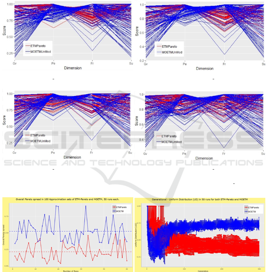
(a) R ID 10 (b) R ID 20
(c) R ID 30 (d) R ID 40
Figure 12: Process models scores on Four quality Dimensions Replay-Fitness(Fr), Simplicity(SU), Generalization(Gv), and
Precision(Pe). The models are obtained by both engines MOETM(Blue), and ETM-Pareto(Red) in runs (R ID) 10, 20, 30,
40.
(a) OS. (b) UD.
Figure 13: (a) is a self-explanatory figure, (b) Generational-Uniform Distribution (UD) (i.e. UD is measured for approxi-
mation sets in every generation not just in the final obtained approximation set) for both engines MOETM(Blue) and ETM-
Pareto(Red) in 100 runs.
Multi-Objective Optimization for Automated Business Process Discovery
101
Process Models Scores on Different Quality
Dimensions and the Pareto Front Shape
(a) Replay-Fitness and Precision.
(b) Generalization and Replay-Fitness.
(c) Simplicity and Replay-Fitness. (d) Replay-Fitness, Precision, and Simplicity.
Figure 14: Process models scores on different quality Dimensions Replay-Fitness, Simplicity, Generalization, and Precision
for models obtained by both engines MOETM(Blue) and ETM-Pareto(Red) in 100 runs along with the pareto front shape.
KDIR 2019 - 11th International Conference on Knowledge Discovery and Information Retrieval
102
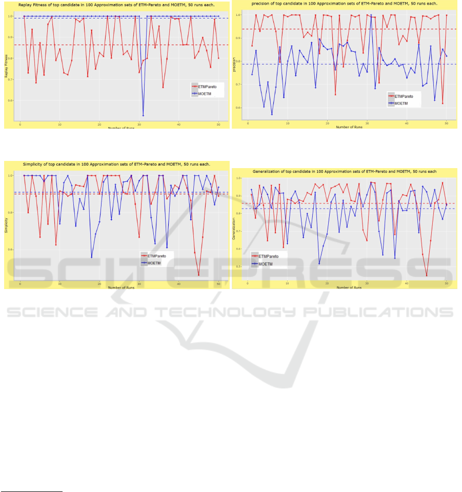
Process Models Scores on Four Quality
Dimensions in All 100 Approximation Sets
Obtained
(a) Replay-Fitness. (b) Precision.
(c) Simplicity. (d) Generalization.
Figure 15: Process models scores on Four quality Dimensions Replay-Fitness(Fr), Simplicity(SU), Generalization(Gv), and
Precision(Pe) of the first candidate (only the first process model happens to exist in the final result) in the 100 Approximation
sets obtained by MOETM and ETM-Pareto.
B: The Weighted Sum Method for MOO
A general Multi-Objective Optimization Problem can
be formulated mathematically as follows:
Minimize
x
F(x) = [ f
1
(x), f
2
(x), . . . , f
m
(x)]
T
s.t x ∈ S
(9)
where m
2
is the number of scalar objective functions
and x is the decision vector with a domain of def-
inition S ⊆ R
n
, where n is the number of indepen-
2
When the number of objectives, m, is more than 3 then
the problem defined by 9 is sometimes also referred to
as many-objective among the evolutionary multi-objective
optimization community.
3
A priori here stand for ”a priori articulation of prefer-
ences” which refers to a set of methods for solving a MOP.
More information on different multi-objective optimiza-
tion methods, and other scalarization techniques can be
found in (Emmerich and Deutz, 2018; Marler and Arora,
2004).
dent variables x
i
, while Z ⊆ R
m
refers to the objective
space and is the forward image of S under the map-
ping F : S → R
m
.
Scalarization techniques are some classical meth-
ods often used in solving MOPs. Scalarizing a MOP
is an a priori method
3
. Briefly, scalarization means
that the objective functions are aggregated or refor-
mulated as constraints then a SOP is solved. By using
different parameters of the constraints and aggrega-
tion function it is possible to obtain different points on
the Pareto front. Various scalarization approaches ex-
ists most notably the weighted sum method. Despite
its well-known drawbacks with respect to depicting
the Pareto optimal set the weighted sum method con-
tinues to be used extensively not only to provide mul-
tiple solution points by varying the weights consis-
tently, but also to provide a single solution point that
reflects preferences presumably incorporated in the
selection of a single set of weights.
Multi-Objective Optimization for Automated Business Process Discovery
103
The Weighted Sum Method
One of the simplest methods for solving a MOP is
to scalarize the problem using a scalarization func-
tion. Many implementations of scalarization func-
tions exist such as the weighted sum, the Chebyshev
scalarization functions, and ε-constraint method. The
weighted sum method is the most common general
scalarization method. Since it is easy to linear weight-
ing by simply attaching non-negative weights to each
objective function and then optimize a weighted sum
of the objective functions using any method for SOO.
In such case the MOP is reformulated to:
Minimize
m
∑
i=1
w
i
f
i
(x), x ∈ S. (10)
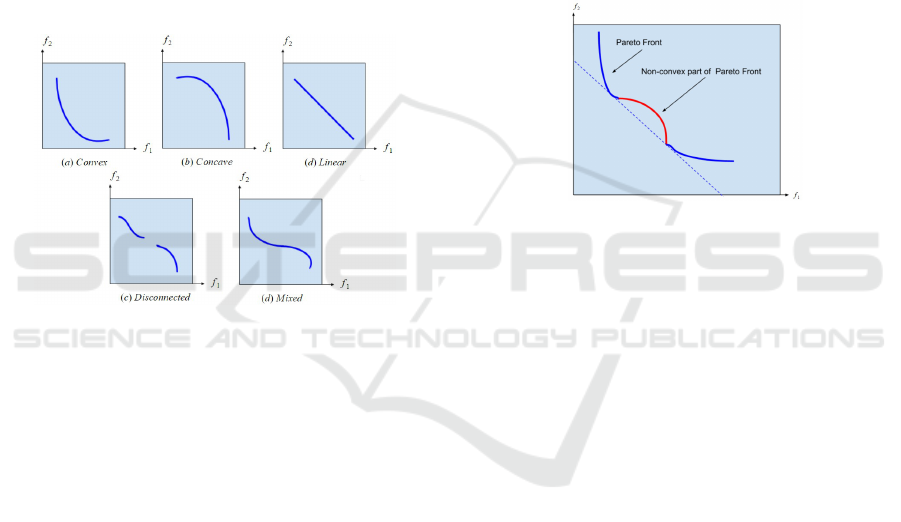
Figure 16: Pareto fronts with different shapes.
In MOO the shape of the Pareto front is an im-
portant property that affects the optimization process.
Since the shape of the Pareto front influences the ef-
fectiveness of multi-objective optimizers which rely
on linear scalarization functions. Generally speak-
ing, figure 16 illustrates five types of Pareto fronts
that can be distinguished depending on their shape:
Convex, Concave, Linear, Disconnected shape, and a
Pareto fronts which contain combinations of the for-
mer shapes. Formal definitions for the notion of con-
vexity and concavity of Pareto fronts can be found in
(Jin, 2012; Emmerich and Deutz, 2018).
In case of a convex Pareto front, possibly all points
on the Pareto front can be obtained by the weighted
sum method. However, if the Pareto front is non-
convex there are points on the Pareto front which
the weighted sum method can not generate. Gener-
ally, in the case of concave Pareto fronts the weighted
sum method will tend to give only extremal solu-
tions, that is solutions that are optimal in one of the
objectives. Figure 17 is an illustration of the non-
convex Pareto front case, the weighted sum method
is unable to obtain solutions in the middle part of
the Pareto front. This well-known drawback of the
weighted sum method along with other drawbacks are
discussed in a number of studies (Marler and Arora,
2004; Emmerich and Deutz, 2018).
Figure 17: Weighted Sum Method unable to find non-
dominated points in non-convex regions of the Pareto front.
KDIR 2019 - 11th International Conference on Knowledge Discovery and Information Retrieval
104
