An MDP-Based Time Domain Impulse Jamming Mitigation Scheme
Yutao Wang
1
, Yingtao Niu
2
, Jianzhong Chen
2
and Fang Fang
1
1
Graduate School, Army Engineering University, Houbiaoying Road, Nanjing, P.R.China
2
The Sixty-third Research Institute, National University of Defence Technology, Nanjing, P.R.China
Keywords: Markov decision process, Anti-jamming, Impulse jamming.
Abstract: This paper proposed a method through a time domain Markov decision process as a countermeasure of
random periodic impulse jamming for a user in a time slotted environment. First, the random periodic
impulse jamming is modelled. Then the time domain MDP-based anti-jamming communication model is
proposed and the optimal transition probability on each state is calculated. Finally, we proposed an online
learning algorithm to approach the optimal transition probabilities. Simulation results show that our method
is better than other countermeasures of impulse jamming.
1 INTRODUCTION
Impulse jamming can corrupt the data transmission
of communication system(Poisel, 2011) in various
applications like IoT systems(Landa et al., 2017),
OFDM systems(Epple and Schnell, 2017) et al. A
short form periodic jamming (SFPJ) attack can cause
huge reduction of packet delivery ratio (PDR) with
little cost and traditional anti-jamming schemes such
as spread spectrum techniques in frequency domain
is not appropriate to the situation due to the impulse
signal has a wide spectrum density(Debruhl and
Tague, 2013). One usual pulse jamming pattern is
called periodic impulse jamming, which generates
impulse jamming periodically. The jamming source
is widely distributed in practice, such as high-
voltage equipment(Lin et al., 2015). Despite the
interferences generated by nature, impulse jamming
is also commonly used by malicious users to corrupt
communication links. Jie et al. derived a closed form
of BER (Bit Error Rate) of optimal periodic impulse
jamming for QPSK system(Jie et al., 2017). As a
countermeasure, the detection of periodic impulse
jamming is studied. Yuan Yuan He, et al.(He et al.,
2008) used wavelet transforming method to estimate
impulse jamming.
Instead of periodic impulse jamming, malicious
user can use variants of periodic impulse jammings
to improve jamming effect and to avoid being
detected. Random periodic impulse jamming is a
kind of impulse jamming whose occurrence time
obeys some distribution. We proposed a Markov
decision process (MDP) based countermeasures to
mitigate the jam effects.
This paper is organized as follow. The system
model is introduced in Section 2. In Section 3, we
calculated the optimal transmission probability
under certain jamming probability. An online
learning algorithm is provided in section 4 to obtain
the optimal transition probability vector. Section 5
presents computer simulation results. Finally, in
Section 6, some concluding remarks are provided.
2 SYSTEM MODEL
Consider the situation where a synchronized time-
slotted communication system consists 2 licensed
users, one of which sender, the other receiver. In
each time slot, the sender sends a frame with length
L
t
. A malicious jamming generates impulse
jamming sequentially with some distributions based
on certain period
,
L
T T t
. We consider each pulse
duration is too short than a frame length, but can
corrupt the frame. In this paper, We assume that the
launched time of
k
’s jamming impulse is
independent normally distributed with a mean of
, 1,2,3,...kT k 
, variance
2

.
Wang, Y., Niu, Y., Chen, J. and Fang, F.
An MDP-Based Time Domain Impulse Jamming Mitigation Scheme.
DOI: 10.5220/0008099500490054
In Proceedings of the International Conference on Advances in Computer Technology, Information Science and Communications (CTISC 2019), pages 49-54
ISBN: 978-989-758-357-5
Copyright
c
 2019 by SCITEPRESS – Science and Technology Publications, Lda. All rights reserved
49



Jamming
Probability
Density
Figure 1: Jamming probability density.
The pdf of the arrival interval is the convolution
of the pdf of 2 adjacent jammings, denoted as
()fx
.
Apparently
()fx
is normally distributed with mean
T
and variance
2
2

. If current time slot is
0
t nT
.
For convenience, we denote the conditional
probability of jamming next time slot is
0
0
max
0
00
0
()
( 1)
()
()
L
tt
t
J
t
t
L
fx
pn
fx
t t t t t
QQ
Tt
Q




  



   











(1)
Where
2
2
2
1
()
2
t
x
Q x e dt





(2)
As a countermeasure which depicted in Figure
2, in each time slot the sender sends a frame
consists 3 elements: payload, verification code
and the Next Action Indicator (NAI). The
verification code part is used to check whether this
frame is corrupted by the jammer, while the NAI
indicates whether to continue send signal or keep
silent next frame, i.e. indicates the receiver
whether a legitimate frame comes next time slot.
We consider the duration of the NAI part is too
small that cannot be influenced by the jamming.
To make the problem clear to understand, we
assume the receiver can immediately sensor the
communication status i.e. whether the channel is
jammed by the malicious attacker.
Payload
Verification Code
Next Action Indicator
Figure 2: Component of a frame.
We define the current the state of the current
time slot
n
S
, At the end of each time slot, the sender
observes the state of the current time slot
n
S
, and
select the corresponding action
{0,1}
n
a 
with a
probability
n
p
, “0” represents “to silent”, “1”
represents “to continue”. When taking action “to
silent”, the sender would stop sending message until
a jamming is detected; when taking action “to
continue”, the sender would continue sending
message next time slot. If this is the Kth consecutive
slot with successful transmission, the state is
denoted by
n
SK
. The transmitter receives an
immediate payoff
()Un
in the nth time slot, decided
by
 
( ) Send (Transmitted) (Jammed)U n R L    1 1 1
(3)
where
R
represents communication gain, while
L
represents jammed loss.
()1
is the indicator
function returns 1 when the statement in the
parenthesis holds TRUE and 0 otherwise.
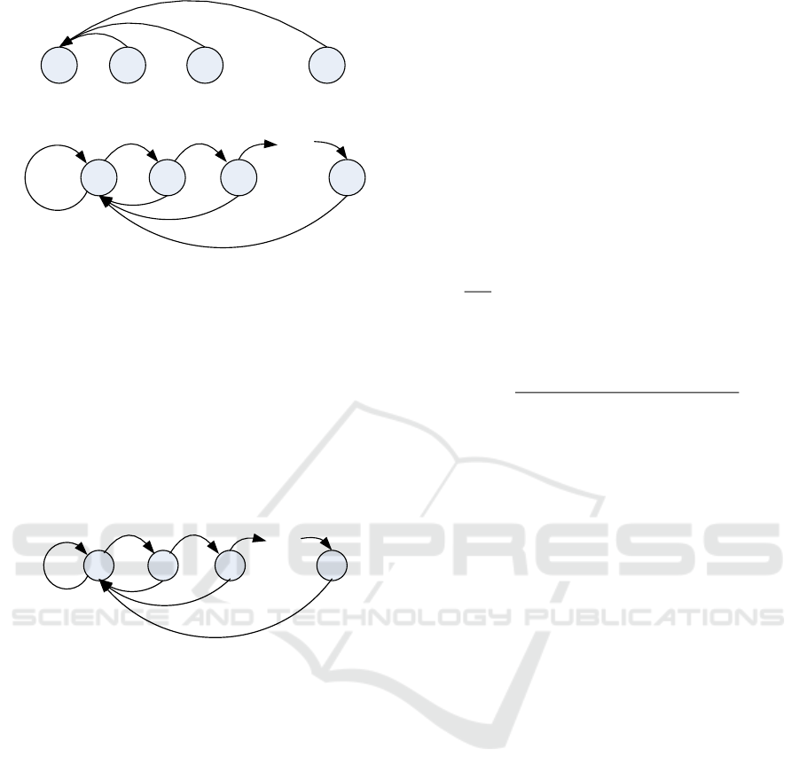
The transition of states can be described as a
Markov chain, as show in Figure 3. The transition
probabilities depend on the action taken by the
transmitter. We use
( ,0|)
mn
P S S
and
( ,1|)
mn
P S S
to represent the transition probability from the
current state
n
S
to a new state
m
S
when taking action
0 and 1, respectively. Obviously,
1
0
0
( | ,1) 1 ( )
( | ,1) ( )
( | ,0) 1, 0
n n J
nJ
n
P S S p n
P S S p n
P S S n




(4)
CTISC 2019 - International Conference on Advances in Computer Technology, Information Science and Communications
50

0 1 2 K
...
0 1 2
K
...
1
1
p
J
(0)
p
J
(1)
p
J
(2)
p
J
(K)
1-p
J
(0) 1-p
J
(1)
1-p
J
(K-1)
(a) Transition of states when taking action silent
(b) Transition of states when taking action continue
Figure 3: Markov chains of state transitions when different
actions are taken.
Note that the jammer may jam the channel with
some probability, the transmitter will have
possibility being jammed when taking action
“continue” at a certain state. The state of the next
time slot depends on the action of the current time
slot, the jamming condition and the state of current
time slot, hence we can model this scenario as a
Markov decision process (MDP), from which the
defense strategy is obtained.
0 1 2
K
...
p
J
(0)
1-p
J
(0)
(1-p
J
(1))p
a
(1) (1-p
J
(K-1))p
a
(K-1)
1-(1-p
J
(1))p
a
(1)
1-(1-p
J
(2))p
a
(2)
1
Figure 4: Total transition probability.
An MDP consists of four important components,
namely, a finite set of states, a finite set of actions,
transition probabilities, and immediate payoffs(Wu
et al., 2011). As the attacker jams the channel with
some distribution, if the transmitter continues
sending message, it will be eventually blocked by
the jammer. Thus, the state
S
will be finite. Denote
the maximum possible According to (3), the
immediate payoff depends on both the state and the
action of previous time slot, i.e.
, if {0,1,2,...}, 1,
( , ) , if {1,2,3,...}, 1,
0, if {0,1,2,...}, 0
nn
n n n n
nn
R S a Unjammed
U S a L S a Jammed
Sa



   




(5)
3 CALCULATION
Our goal is to find the appropriate
a
p
that can
maximize the sum of immediate payoff and expected
payoff conditioned on the current action probability.
1
( ) ( , )
N
nn
n
U U S a



S
(6)
In all the scenarios above, the interval between 2
jamming signals is not infinite in practice, so we can
be informed that the states are also finite. Denote
max
L
t
N
t




as the maximum states count, where
max
()
thresh
f t p
.
( | )
()
(|)
L L L L
J
LL
f t n t t n t t t n
pn
f t t n t t n
      

   
(7)
Denote
01
( , ,... )
N
S S SS
which represents state
vector,
01
( , ,... )
N
a a aa
represents action vector;
( (0), (1),... ( ))
S S S
p p p N
S
p
represents vector of
probabilities of each state;
( (0), (1),... ( ))
a a a
p p p N
a
p
represents vector of
probabilities of action on each state;
( (0), (1),... ( ))
J J J
p p p N
J
p
represents vector of
jamming probability on each state.
From the definition,
(0) 1
a
p 
,
( ) 1
J
pN
,
( ) 0
a
pN
. With the transition probability
a
p
we
can derive the total state transition probability matrix
P
.
   
 
1 1 (0) (0) 1 (0) (0) ... 0
1 1 (1) (1) 0 ... 0
... ... ... ...
1 0 ... 0
J a J a
Ja
p p p p
pp

  














P
(8)
Proposition 1: The states probability
S
p
is
determined by
J
p
and
a
p
.
Proof: from (8), the following stationary
distribution of the Markov chain can be formulated
as below:
 P
SS
pp
(9)
An MDP-Based Time Domain Impulse Jamming Mitigation Scheme
51

0
0
01
12
1,
(0) ( )
(1) (0)
(2) (1)
...
( ) ( 1)
N
S n S
n
SS
SS
S N N S
p p p n
p p p
p p p
p N p p N







(10)
Subject to
0
( ) 1
N
S
n
pn



(11)
mn
p
denotes the transition probability of state
m
to
n
. Thus, the states’ probability can be figured out
as
,1
10
(0) ( ) 1
Nn
S S k k
nk
p p n p




  





(12)
According to (8)(10)(12),
 
   
1
,1
10
1
(0)
1
(1) 1 (0) (0)
...
( ) 1 (0) ... 1 ( 1) (0)
S
Nn
kk
nk
S J S
S J J S
p
p
p p p
p N p p N p












     

(13)
Thus, the states’ probability
S
p
can be
determined by
J
p
and
a
p
.
The returning to state
0
S
from state
0
S
through
several states is defined as a cycle. It is obvious that
the state will eventually return to
0
S
. The total
probability from each path in a cycle is 1, i.e.
0 1 0
0
Pr{ ... } 1
N
k
k
S S S S



(14)
The expectation of total payoff in one cycle is
denoted as
*
()U S
, which can be obtained by the
equation below.
 
*
0
()
( ) ( )( )
(0)
()
()
1 ( )
(0)
S
aJ
N
S
n
S
a
S
pn
p n p n nR L
p
U
pn
p n nR
p





















  








S
(15)
From the equation, it can be inferred that
*
()U S
is determined by
a
p
and
J
p
. Our algorithm aims to
achieve the goal of maximizing
*
()U S
, the
following equation is needed.
 
 
*
0
argmax ( )
()
( ) ( )( )
(0)
argmax
()
1 ( )
(0)
S
aJ
N
S
n
S
a
S
U
pn
p n p n nR L
p
pn
p n nR
p




















  









a
pS
(16)
It is theoretically possible to calculate the
optimal
a
p
. However, the calculation is too
complex to solve due to
a
p
is a
max
L
t
t



dimension
vector. If the probability resolution is
dp
, the
solution space will be
max
1
L
t
t
dp









. To find the max
value and its index in acceptable time, the Simulated
Annealing Algorithm(Ogbu and Smith, 1990) is
introduced into this model. We set the vector
a
p
as
argument. At each epoch, we make a random change
of
a
p
and compare the expectation of corresponding
*
()U S
. The change is accepted according to
metropolis criterion. After sufficiently large time,
the probability of
 
*
argmax ( )U
a
pS
will be 1.
4 ONLINE LEARNING APPROAH
In practice, the jamming probability vector
J
p
cannot be obtained from the environment
immediately. To approach the optimal transition
probability vector
a
p
, We propose an online
learning algorithm. According to the simulation
results, the optimal
{0,1}
a
p
, and all “1” occur
before a certain time slot and all “0” after that
certain time slot. So we translate the problem into
find this certain time slot as boundary before which
CTISC 2019 - International Conference on Advances in Computer Technology, Information Science and Communications
52

continuously transmitting signal. We formulate the
problem as a multi-armed bandit problem. The user
selects Kth arm represents continuously transmit
K
time slots. Facing this problem, the trade-off
between exploration and exploitation is the focus of
the problem. If the user chooses the exclusively on
the arm that he thinks is best(exploit), he may miss
the actual best arm. If the user keeps trying out all
the arms and gathering statistics (“exploration”), he
may fail to play the best arm often enough to get a
high return(Auer et al., 2011).
We define 2 variables, exploration rate

and
temperature
t
to solve the problem. Both the two
variables decrease over iteration. If the exploration
rate is higher, the user is more likely to choose the
new state to calculate the new payoff and vise versa.
If the temperature is higher, the user is more likely
to accept the new arm and vice versa.
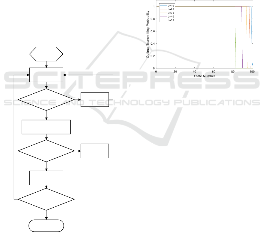
The user selects the first arm at first transmitting
cycle and calculate the sum payoff according to
actual jammings. Our algorithm is depicted as
Figure 5.
Init: , 
Calculate 


Update 
according to 


  




    


Update  
Convergence?
Update 
according to 
Calcuate 

  
according to 
end
Y
N
Y
N
N
Y
Figure 5: Online learning algorithm to approach optimal
boundary.
5 SIMULATION RESULTS
First, we calculated the effect of different parameters
to transmitting probability
a
p
. We set transmission
gain
10R 
, time slot length
0.01
L
ts
. For a
normal distributed jamming, the jamming period
0.5T 
and variance
22
0.1


. With different
10,20,30,40,50L 
. The result is shown in Figure 6.
The transmitting probability goes from 1 to 0 with as
sharp gradient. Different jamming loss result in
different transmitting probability vector. With
greater jamming loss, the transmitting time slot
trends to be shorter.
Figure 6: Optimal transmitting probability with different
jamming loss with
22
0.1


.
In Figure 7, we compared our scheme with
different combinations of the attack and the defense
strategy. The transmission gain and jamming loss
are set to 10 and 30 respectively. We plotted the
average sum payoff of a cycle in all the 5 situations.
First, the communication is under a non-jamming
environment. The equivalent average sum payoff of
a cycle is the highest. After that, a periodic impulse
jamming occurs and makes the average sum payoff a
great loss. As a countermeasure, the authorized user
takes periodic transmission to withstand the impulse
jamming. The malicious attacker then chooses
random periodic impulse jamming strategy, which
drops the average sum payoff most. To mitigate the
jamming effect, the authorized user then chooses
MDP-Based impulse jamming mitigation scheme
that rises the average sum payoff curve.
An MDP-Based Time Domain Impulse Jamming Mitigation Scheme
53

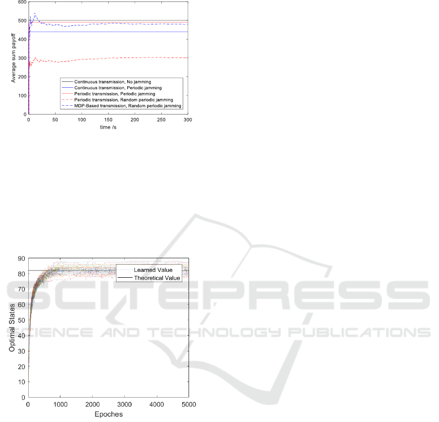
Figure 7: Comparison of different anti-jamming schemes.
In Figure 8, the proposed algorithm in section 4
is verified. We generated normally distributed
jamming with a mean of
, 1,2,3,...kT k 
,
0.5T 
,
variance
2
0.1


. Transmitting gain
10R 
,
jamming loss
50L 
. The theory value optimal state
is calculated based on optimal
a
p
obtained at the
beginning of this section.
Figure 8: Comparison between learned value and
theoretical value.
6 CONCLUSIONS
In this paper, we proposed a Markov decision
process based impulse jamming mitigation scheme
and used simulated annealing algorithm to obtain the
numerical result. The optimal transmitting
probability is either 0 or 1, and the continuously
transmission slot is shorter when jamming loss
L
grows. We have shown that our scheme is better
than periodic transmission scheme under same
random periodic impulse jamming environment.
REFERENCES
Auer, P., N. Cesa-Bianchi, Y. Freund and R. E.
Schapire, 2011. The Non-Stochastic Multi-
Armed Bandit Problem. In Siam Journal on
Computing 32(1):48-77.
Debruhl, B. and P. Tague, 2013. How to jam without
getting caught: Analysis and empirical study of
stealthy periodic jamming. In IEEE International
Conference on Sensing.
Epple, U. and M. Schnell, 2017. Advanced Blanking
Nonlinearity for Mitigating Impulsive
Interference in OFDM Systems. In IEEE
Transactions on Vehicular Technology
66(1):146-158.
He, Y. Y., C. J. Yu, T. F. Quan and X. Jin, 2008.
Impulsive interference detection method based
on Morlet wavelet and maximum likelihood
estimation. In IEEE International Conference on
Industrial Informatics.
Jie, Y., H. Bingyang and X. Jingying, 2017. Optimal
Periodic Pulse Jamming Signal Design for QPSK
Systems. In Journal of Beijing Institute of
Technology 26(3):381-387.
Landa, I., A. Blazquez, M. Velez and A. Arrinda,
2017. Indoor measurements of IoT wireless
systems interfered by impulsive noise from
fluorescent lamps. In European Conference on
Antennas & Propagation.
Lin, J., T. Pande, I. H. Kim, A. Batra and B. L.
Evans, 2015. Time-Frequency Modulation
Diversity to Combat Periodic Impulsive Noise in
Narrowband Powerline Communications. In
IEEE Transactions on Communications
63(5):1837-1849.
Ogbu, F. A. and D. K. Smith, 1990. The application
of the simulated annealing algorithm to the
solution of the n / m / C max flowshop problem.
In Computers & Operations Research 17(3):243-
253.
Poisel, R. A., 2011. Modern Communications
Jamming Principles and Techniques, Artech
House, Inc.
Wu, Y., B. Wang, K. J. R. Liu and T. C. Clancy,
2011. Anti-Jamming Games in Multi-Channel
Cognitive Radio Networks. In IEEE Journal on
Selected Areas in Communications 30(1):4-15.
CTISC 2019 - International Conference on Advances in Computer Technology, Information Science and Communications
54