Optimization of Software Estimation Models
Chris Kopetschny
1
, Morgan Ericsson
2 a
, Welf L
¨
owe
2 b
and Anna Wingkvist
2 c
1
Dezember IT GmbH, Edenkoben, Germany
2
Department of Computer Science, Linnaeus University, V
¨
axj
¨
o, Sweden
Keywords:
Estimation Models, Optimization, Software Engineering.
Abstract:
In software engineering, estimations are frequently used to determine expected but yet unknown properties of
software development processes or the developed systems, such as costs, time, number of developers, efforts,
sizes, and complexities. Plenty of estimation models exist, but it is hard to compare and improve them as
software technologies evolve quickly. We suggest an approach to estimation model design and automated
optimization allowing for model comparison and improvement based on commonly collected data points.
This way, the approach simplifies model optimization and selection. It contributes to a convergence of existing
estimation models to meet contemporary software technology practices and provide a possibility for selecting
the most appropriate ones.
1 INTRODUCTION
Several software engineering steps depend on estima-
tions, e.g., estimating the complexity and the effort
for implementing a particular task or estimating the
time and costs of implementing a system. Conse-
quently, there are plenty of methods and models sug-
gested for these estimation tasks. We will introduce
known methods and models for software estimation
and continue with problem description and analysis
to end the introduction presenting our research aims.
1.1 Known Methods and Models
There are plenty of known software estimations mod-
els, e.g., COCOMO, the first version known as CO-
COMO 81 and the second as COCOMO II (Boehm
et al., 2009), COSYSMO (Valerdi, 2004), Evidence-
based Scheduling (a refinement of typical agile esti-
mating techniques using minimal measurement and
total time accounting) (Spolsky, 2007), Function
Point Analysis (Albrecht, 1979), Parametric Estimat-
ing (Jenson and Bartley, 1991), Planning Game (from
Extreme Programming) (Beck and Andres, 2004), the
ITK method (also known as the CETIN method),
Proxy-based estimating (PROBE, from the Personal
a
https://orcid.org/0000-0003-1173-5187
b
https://orcid.org/0000-0002-7565-3714
c
https://orcid.org/0000-0002-0835-823X
Software Process) (Humphrey, 1996), Program Eval-
uation and Review Technique (PERT) (Office, 1962),
the Putnam model (also known as SLIM) (Putnam
and Myers, 1991), the PRICE Systems (commer-
cial parametric models that estimates the scope, cost,
effort and schedule for software projects), SEER-
SEM (Galorath and Evans, 2006) (parametric estima-
tion of effort, schedule, cost, risk.) Minimum time
and staffing concepts based on Brooks’s law (Brooks,
1995), the Use Case Points method (UCP) (Karner,
1993), Weighted Micro Function Points (WMFP),
and Wideband Delphi
1
.
1.2 Problem Description and Analysis
Modern software technology advances at a fast pace
including development tools and environments, plat-
forms, reusable components and libraries, languages,
and processes. What is appropriate software technol-
ogy today might be outdated in the near future. There-
fore, also the estimation models need to change at the
same speed because, otherwise, they become outdated
and, hence, imprecise for modern software develop-
ment.
Cloud technologies used in software development
have the potential to provide us with access to pre-
viously unknown amounts of data, i.e., Big Data.
1
https://en.wikipedia.org/wiki/Cost estimation in soft
ware engineering
Kopetschny, C., Ericsson, M., Löwe, W. and Wingkvist, A.
Optimization of Software Estimation Models.
DOI: 10.5220/0008117701410150
In Proceedings of the 14th International Conference on Software Technologies (ICSOFT 2019), pages 141-150
ISBN: 978-989-758-379-7
Copyright
c
 2019 by SCITEPRESS – Science and Technology Publications, Lda. All rights reserved
141

Converted into actionable knowledge, data has be-
come an unprecedented economic value as witnessed
by the success of companies like Google, Facebook,
and Twitter. Big Data has also revolutionized soft-
ware engineering research and its scientific method-
ologies leading a paradigm shift away from data-
scarce, static, coarse-grained, and simple studies to-
wards data-rich, dynamic, high resolution, and com-
plex observations and simulations.
However, Big Data has not yet been fully ex-
ploited in estimation model building, validation, and
exploitation. One reason might be that the relevant
data is distributed among different stakeholders in an
organization, e.g., relevant impact factors of devel-
opment time are task complexity (estimated by the
development team), team competence and availabil-
ity (assessed by the personnel lead), and processes
and environment maturity (evaluated by a CTO). An-
other reason might be that the relevant data becomes
available at different points in time. For instance, the
aforementioned factors of estimation are available be-
fore the project starts, while the actual ground truth
only gets available afterward. Further to complicate
matters, data points can be generated in different or-
ganizations and, hence, are hard to collect and to ex-
ploit commonly.
As a consequence, we face a lot of shortcomings
in the currently suggested estimation models, despite
all benefits of cloud and Big Data technologies. Es-
timation models are built from prior data collected
years before and looking at software development
practices of today; they are outdated. Consequently,
they emphasize factors that are nowadays irrelevant
and neglect factors of high contemporary importance.
The model constants of these models are often out-
dated too and cannot be adapted to today’s technolo-
gies without significant effort. There is no automatic,
continuous learning and improvement.
The models are incomplete, e.g., they estimate the
size but not the effort, or estimate the effort based on
the size but do not estimate the size itself. They are
also incompatible with each other, i.e., they require
similar, though not identical, factors. As an example,
the development environments and product factors are
regarded both to impact on the estimated system size
and the development effort, which gives these factors
too high weights overall.
Developing new estimation models is not a solu-
tion to the aforementioned shortcomings if the pro-
cess of their development would not change. We
claim that the estimation model development faces
some inherent problems. New models cannot be
tested without a significant cost in time and effort.
The errors and, hence, the suitability of these mod-
els cannot be calculated automatically and in a uni-
versal way. Also, some estimation factors, e.g., pa-
rameters of a project, partially overlap, are dependent
on each other, i.e., they correlate. If the correlation is
strong, they are redundant and therefore, superfluous.
To date, this can only be recognized and optimized
with a manual effort, if done at all.
To train a new model, more data points have to be
collected first. Given the fact that there are often not
enough data points available or they do not exist in a
uniform structure because no uniform process exists
for collecting the data we face a so-called “cold start
problem”. This leads to a lot of effort for data collec-
tion and model estimation before gaining any value.
However, even imprecise objective estimation models
have a value compared to and complementing subjec-
tive assessments.
1.3 Research Aims
This research contributes with an approach to test
and improve estimation models mapping, e.g., cost
drivers to costs. The approach shall be agnostic with
respect to the specific domain and help to test and im-
prove models for mapping any indicator of an out-
come to the actual outcome.
Additionally, the following requirements shall be
met: The approach is data-driven and improves with
newly available data points. In such an approach, new
model ideas should be easily trained and tested with
old data points. New models should coexist and com-
pete with previously defined models. The approach
supports the calculation and comparison of the accu-
racy of all competing models based on all data points
and adjusts the parameters of each model to minimize
potential errors. The approach should also be under-
standable by human experts.
The goal of this work is not to develop one or
more concrete, accurate estimation models. Because
of the cold start problem and the fact that nowadays
technologies change faster, simultaneously makes the
continuous learning of the coefficients more impor-
tant, our approach should help improve models and
increase their accuracy over time. Moreover, it should
not matter what a model looks like, i.e., what class
of functions it exploits nor its domain. Instead, the
approach shall be universal. If sufficient initial data
points are available, arbitrary models can be tested,
trained, iteratively improved, and eventually used.
The following research questions guided our
work:
RQ1 How can we define a continuously improving
approach where new models are easy to imple-
ment, validate, and adjust?
ICSOFT 2019 - 14th International Conference on Software Technologies
142

RQ2 How can data points be collected while detect-
ing correlations and dependencies between inputs
while avoiding unnecessary inputs?
RQ3 Can we automate the approach?
In short, instead of suggesting the one and only
model for estimations we aim at establishing an ef-
fective and efficient process to collect data points and
develop different competing estimation models based
on these data points that are useful at any point in time
and that converge to more and more accurate tools.
We rely on a design science approach (Simon,
1996) and formulate the goal criteria as well as the
design of our approach in Section 3. We evaluate an
implementation of our approach in Section 4 against
these goal criteria and discuss how well these are ful-
filled in Section 4.5. In Section 5, we present our con-
cluding remarks and our thoughts on future work.
2 THE COCOMO FAMILY OF
SOFTWARE ESTIMATION
MODELS
While our approach is agnostic to the actual estima-
tion problem and the model to estimate, we still want
to introduce a concrete model as an example for better
relating to the issues and challenges.
The Constructive Cost Model (CO-
COMO) (Boehm et al., 2009) is arguably still
the most widely used software implementation effort
estimation model. It can also be applied to estimating
the re-implementation effort. It was developed in
1981 and last updated with “new” calibration data—
only 161 data points—in 2000. It aims at estimating
the effort E in person months depending on the esti-
mated project size N in lines of code and on different
project and team parameters. Different model input
parameters—so-called effort multipliers (em) and
scale factors (sf)—have an impact on the estimated
effort E, such as Development Flexibility, Team
Cohesion, and Software Cost Drivers, which are then
subdivided into Product, Personnel, Platform, and
Project Cost Drivers.
The model is weighted with model constants a and
b that need to be calibrated using data points from real
projects. These are the formulas behind COCOMO:
E = a × (N/1000)
e
×
17
∏
i=1
em
i
e = b × 0.01 ×
5
∑
i=1
sf
i
Similar to COCOMO, the Constructive Systems
Engineering Cost Model (COSYSMO) uses the size
of a system and adapts it according to the correspond-
ing parameters. It was developed in 2002 and was cal-
ibrated with approximately 50 projects. It estimates
person months as a function of the four size parame-
ters: number of system requirements, number of sys-
tem interfaces, number of algorithms, and number of
operational scenarios (Valerdi, 2004).
With COCOMO and COSYSMO software engi-
neers can estimate certain cost driving factors (inde-
pendent variables), for example, lines of code, and
then apply the model to estimate time and costs
(dependent variables). Since the function classes
for mapping independent to dependent variables are
known, regression of the function parameters can
be done and redone. However, currently suggested
parameters are originally trained on very few data
points.
Based on the same data points, there is no possi-
bility to create, test, and optimize parameters of new
models, since the relevant independent variables and
the function class of the model are static. The mod-
els are outdated and do not regard today’s practices
in software developments, for example, new develop-
ment processes like the agile approach. The projects
on which COCOMO is based are all realized with the
waterfall concept. It seems that COCOMO overesti-
mates the effort since some cost drivers that had a high
impact back in the time when they been defined are
less important now. They are less influential nowa-
days due to technological progress, e.g., larger scale
projects are easier to manage today than in 2000. In
short, COCOMO and COSYSMO do not have any
function type calibration capabilities and do not con-
sider the addition of new parameters. At best, these
models could provide an upper bound of the poten-
tially achievable accuracy.
A recent study on effort estimation found that if
a project gathers COCOMO-style data, none of the
newer estimation models did any better than CO-
COMO (Menzies et al., 2017). They conclude that
if such data were available, it should be used together
with COCOMO to perform predictions.
The upcoming COCOMO III was first announced
in 2015 (Clark, 2015) and should consider the scope
of modern software. Especially, new development
paradigms, new software domains like Software as a
Service, mobile, and embedded as well as big data
should be addressed. It should improve the realism
and contain new and updated cost drivers. Unfortu-
nately, the announcement has been out for a long time,
and it is not known when or if at all, COCOMO III
will ever be released.
Optimization of Software Estimation Models
143

It is not easy to keep old models updated or sug-
gest new models, prove them superior, and abandon
the previous ones.
3 ESTIMATION MODEL
DEVELOPMENT
3.1 From Informal Requirements to
Measurable Goal Criteria
The goal of this work is to help users develop models
that improve over time. Model developers can thus
add models. Along with new data points being added
continuously, the accuracy of the model should im-
prove. It should not matter what a model looks like,
i.e., what class of functions it exploits or what domain
it has. Instead, the approach should be universal; if a
sufficient number of initial data points are available,
arbitrary models can be tested, trained, iteratively im-
proved, and eventually used. We define the following
Goal Criteria (GC) for our solution refining the re-
quirements posed in Section 1.3:
GC 1: The models should be able to make pre-
dictions based on learning from available data.
Therefore, a suitable approach would allow col-
lecting data points in central data storage and a
consistent format. Data should be cleaned up, and
it should be possible to deal with missing data val-
ues.
GC 2: The accuracy of the predictions should im-
prove continuously through model optimization.
GC 3: Possible model improvements should be sug-
gested automatically, e.g., if some parameters in a
model become superfluous.
GC 4: It should be possible to determine if a pre-
diction is trustworthy, e.g., by determining if it is
based on outlier data.
GC 5: The models should be possible to inspect and
be understandable by human domain experts. The
influence of specific inputs on the result should be
recognized.
GC 6: The approach should be universally applica-
ble to any models and domains.
Further note that machine learning is often used to
create models that can make predictions based on in-
put data. However, these models are generally “black
boxes” that are difficult to understand and learn from.
Hence, while machine learning would fulfill some
of the goal criteria, it would violate GC 3 and 5.
Machine learning models also often exclude princi-
ple function classes and may result in over-trained or
over-fitted models, especially when only a few data
points are available. We instead rely on “white box”
models. Designed parametric models that are explic-
itly defined based on expert domain knowledge, e.g.,
within software project management. While these
might perform worse compared to machine learning
models for some goal criteria, such as 2, they do ful-
fill all goal criteria.
3.2 Mathematical Foundations
A parametric model is provided as a function, e.g.,
Y = f (x) = a ×X +b, where X is an input parameter,
a and b are parameters, and Y is an estimate. A data
point consists of tuples of input variables and their
corresponding, ideally correct estimates, e.g., (x,y)
with x being an X value and y being a Y value. The
objective of the model optimization is to determine
values for the parameters, so that they provide the best
possible accuracy for the observed data, i.e., to min-
imize the mean squared error, (y − (a × x + b))
2
, for
all data points (x,y).
The main step is to train the parameters of a
human-developed model. Note, that since the model
formulas are not always linear, linear regression gen-
erally cannot be used. Non-parametric regression is
also not applicable either since the goal is not to find
the parametric model. It would result in a model that
is massively over-trained, especially in the light of the
aforementioned cold start problem. It would also be
too complex to be understandable.
Optimization algorithms can calculate the mini-
mum or maximum of a massively over-determined
system of equations and, therefore, optimization al-
gorithms for zero-point calculations should be used.
Various groups of optimization algorithms exist for
this purpose. We classify them based on which
derivative they need: class A requires the second
derivative and class B only the first derivative. For
example, Gradient descent requires the first deriva-
tive and is thus of class B while the Broyden-Fletcher-
Goldfarb-Shanno algorithm requires the first and sec-
ond derivatives and is of class A.
In practice, derivatives of the model function do
not always exist, because not all model functions
can be differentiated at every argument vector. If no
derivations are known, only optimization algorithms
for non-differentiable functions can be used to deter-
mine constants. We, therefore, define a class C where
no derivative is used, e.g., the Downhill Simplex al-
gorithm.
In our implementation, we currently consider the
ICSOFT 2019 - 14th International Conference on Software Technologies
144

following five optimization algorithms: Broyden-
Fletcher-Goldfarb-Shanno (A) (Fletcher, 1987),
Quasi-Newton (A) (Huang, 2017), Gradient descent
(B), Downhill simplex (C) (Nelder and Mead, 1965),
and Trust-region (C) (Sorensen, 1982). Note that
our system is extensible with any number of such
algorithms.
3.3 Optimizing Model Parameters and
Assessing Models
Our approach contains the following steps. Data
points are continuously collected, and domain experts
develop and add models. Based on the data points,
optimization algorithms are used to determine the pa-
rameters in the models that best fit the collected data
points. To determine the performance of the various
models, the error is calculated and based on this er-
ror, we determine whether the model can be used for
predictions or not. Finally, it is suggested how the
models can be improved.
The model function is entered manually in our ap-
proach. Then an algorithmic differentiation is used
to try to determine the derivatives automatically. If
this is successful, the corresponding optimization al-
gorithms of class A and B are available for finding the
constants. If not, the approach asks for manual enter-
ing of the first and second derivatives of a model. If
the model developer does not want to or cannot pro-
vide them only optimization algorithms of class C can
be used.
All optimization algorithms that can be used for a
suggested model, depending on the available deriva-
tions, belong to the “pool of available algorithms” and
are used for subsequent optimizations of the corre-
sponding model. For example, a model for which the
second derivative is defined, the pool consists of op-
timization algorithms from classes A, B, and C. Each
model function is optimized for all applicable data
points using all optimization algorithm from the pool.
The set of applicable data points consists of all
data points that have corresponding values for all in-
put variables occurring in the model. If a model func-
tion requires an input x, and this is not contained in
a data point, this data point is not used for optimiza-
tion. If, on the other hand, input x = N/A, i.e., it was
requested but not provided, standard procedures from
statistics are used to deal with missing data and the
data point is used. In the simplest case, the missing
data are replaced with the mean value, no matter what
kind values were missing. Other statistical standard
methods like regression imputation, substitution by
positional dimensions, or maximum likelihood meth-
ods can also be used.
Assume an existing model M is manually im-
proved and saved as M
0
. If M
0
contains at most the
input variables of its predecessor M then existing data
points could be used to train the new model as well.
This is because these data points include all input
variables needed to train M and are, hence, applicable
also for M
0
. This makes the two models comparable
directly. Conversely, if M
0
adds a new input variable,
it is critical to apply the standard procedures for deal-
ing with missing data in M and to compare M and M
0
based on existing data points.
If the error functions are convex then it is easy to
find the global minimum. If they are not convex, it is
potentially difficult to find the global minimum. It is,
however, enough to find several local minima and se-
lect the best of these. In addition to the application
of various optimization methods, various measures
should be taken to increase the probability of find-
ing different local minima to choose the best from.
These measures include learning parameters to make
larger or smaller jumps, the addition of random val-
ues to weights, and the use of Momentum Terms to
add to past weight adjustments, 0.25, 0.125, etc. All
this remains transparent for the model developer.
All optimization procedures contained in the pool
of available algorithms are applied several times with
different settings, and each suggests parameters. Then
it is checked which of these produces the best result,
i.e., the smallest errors.
In the first step, the parameters for each given
model are calculated with each implemented opti-
mization algorithm and all data as training data.
These parameters are potentially over-optimized. For
error calculation, we calculate the mean squared er-
ror mse, i.e., the distance between Y
calc
and Y
real
is
calculated, squared, and averaged, cf. Equation 1.
mse =
1
n
n
∑
i=1
(Y
calc
i
−Y
real
i
)
2
(1)
In the second step, the principles of cross-
validation are used. Iteratively, the data points are ran-
domly divided into training and test data sets. Then,
the parameters are calculated from the training data,
and the corresponding error is calculated from the test
data according to equation 1. For each iteration, the
calculated errors may differ. Therefore, the errors are
averaged out. This is done until the change in the av-
eraged error is smaller than ε constant or after a fixed
number of iterations. The latter is an emergency stop
function guaranteeing termination that is used when-
ever the parameters found are not stable.
The following data is stored for each run: the
model, optimization algorithm, the algorithm setting,
the parameters, the mean squared error for the train-
Optimization of Software Estimation Models
145

ing session, the averaged mean squared error for the
testing data sets, and a list of the data points used.
3.4 Improving Models
The calculated models might have a large number of
input variables, which may be very time-consuming
to retrieve and to enter. It is possible that 30 out of 50
input variables in a model function can explain 95%
of the information gain. A human expert can then im-
prove the model so that in the future, only the relevant
variables need to be assessed and entered. For exam-
ple, if two variables are linearly highly dependent on
each other, then one of the two can be omitted. Our
approach supports this manual model improvement.
Principal Component Analysis (PCA) forms the
basis for calculating the information gain of input
variables. After each parameter optimization, it can
give hints on model improvements. Therefore, Eigen-
values and Eigenvectors are calculated. The Eigenval-
ues indicate how significant the respective Eigenvec-
tors are for the explanatory power. The Eigenvalues
corresponding to a component divided by the sum of
all Eigenvalues gives the information gain of the re-
spective component. First, the principal component
is calculated. After that, it is calculated how good
the principle component replacement is. Finally, the
input variables are ranked based on their explanatory
power.
a
1
× X
2
1
+ a
2
× X
2
+ a
3
(2)
Based on the indication for the explanatory power
of an input variable, the model developer is usually
interested in how the model behaves if input variables
or even complete terms are omitted. To avoid creat-
ing a new model for each such constellation, individ-
ual terms and parameters can be “switched off” semi-
automatically. For example, the parametric model
given in Equation 2 can be entered with optional parts.
Three different alternatives are shown in the Equa-
tions 3a–3c.
a
1
∗ X
2
1
+ Ja
2
× X
2
+Ka
3
(3a)
a
1
× X
1
J
2
K + a
2
× X
2
+ a
3
(3b)
Ja
1
×KX
2
1
+ Ja
2
×KX
2
+ a
3
(3c)
Brackets [[·]] are used to indicate optional parts.
The terms between an opening and a closing square
bracket are included in the model. However, a model
developer can optionally skip them during the param-
eter optimization steps. The errors of the different op-
tions of the model formula can always be compared
with each other. It would also be feasible to work
with neutral and inverse elements, but this is not that
flexible, since the expression of the inverse element
is often complicated, and the optimization time grows
because more variables need to be evaluated.
3.5 Using Models
With a trained parameterized model, it is in principle
always possible to make predictions. Depending on
their accuracy, they can be a complement to or a sub-
stitute for human based, subjective estimations. To do
that, a data point for which the estimate is not known
can be entered. Then a predicted value is calculated,
always using the best constants of the best applicable
model.
Using the results of a trained model only works re-
liably if the designed parametric model is suitable in
the first place and if the data points collected are suit-
able. Suitability of the model means that it reflects the
actual relation between input and estimation variables
and only disregards the actual parameter value. Suit-
ability of the data points means that they are repre-
sentative samples of the real-world development pro-
cesses. Then, over time, the errors tend to decrease
with new data points.
The model designer is responsible for assessing
the suitability of the model. Regarding the suitabil-
ity of a data point, statistical methods can support the
model designer: Assuming that the input variable val-
ues are generally normally distributed and are within a
scattered range around the expected value, values fur-
ther than, e.g., two times the standard deviation out-
side the expectation could be regarded as outliers. If
the variable values are not normally distributed, other
criteria must be defined in order to distinguish be-
tween outliers and non-outliers. For run time effi-
ciency, a standard data-mining algorithm should be
used in practice, e.g., the Local Outlier Factor Algo-
rithm (Breunig et al., 2000), which does not depend
on the normal distribution.
4 EVALUATION
We experimentally investigate GC 1 and GC 2,
whether the parametric models can be parameterized
automatically based on data, become more and more
accurate, and that the errors converge.
4.1 Implementation
Therefore, we implemented the approach as a web ap-
plication with a simple CRUD-interface in Laravel
ICSOFT 2019 - 14th International Conference on Software Technologies
146

and PHP to enter data points and models. These were
stored in a MySQL database and all optimizations were
implemented using R, specifically the optim and nlm
functions. To make the application portable, we pack-
aged it as a Docker container.
4.2 Training Data and Models for
Evaluation
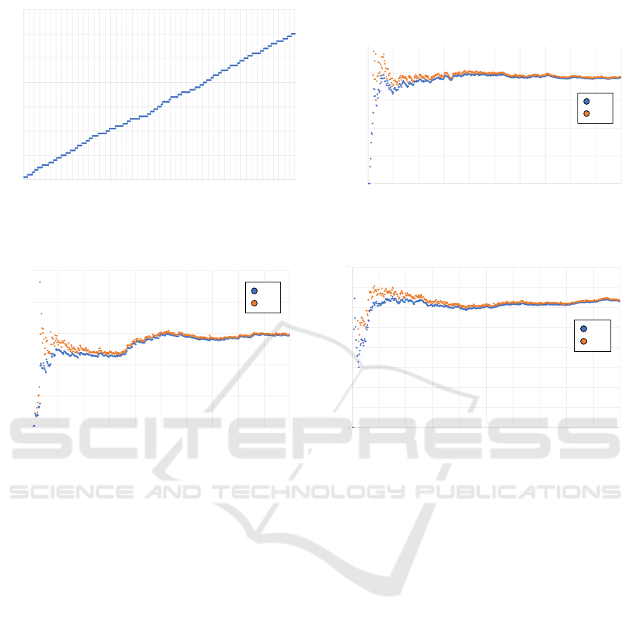
We use synthetic data and artificial models to eval-
uate, since the focus is on evaluating whether the
approach fulfills the goal criteria, not to create real-
istic and useful models per se. In the evaluations,
we use three data generators: d
1
(x) = A × x + B,
d
2
(x) = A × x
3
+ B, and d
3
(x) = A × sin x + B. The
data points in these data sets are generated by placing
random seed constants into a model so that the real
fuzziness is simulated, cf. Figure 1 for the first data
set.
We also use three parametric estimation models:
f
1
(x) = a × x + b, f
2
(x) = a × x
3
+ b, and f
3
(x) =
a × sin x + b.
The approach should fit a to A and a to A when
optimizing the first (second, third) model with the first
(second, third) data set.
4.3 Experiments and Evaluation
Method
4.3.1 One Model and Several Data Sets
We first investigate a single model, f
1
(x) and three
different data sets generated from d
1
, d
2
, and d
3
. We
generate data randomly for each data sets, optimize
the parameters a, b of the model f
1
(x). The model
optimization should fit the model to minimize the er-
ror. As discussed previously, we compute two errors,
e
1
that uses all data points as the training set and e
2
that uses a cross-validation approach and divides the
data set into training and test sets. Both are calculated
as the mean squared error. For each new data point
randomly generated, we assess these errors.
4.3.2 Several Models and One Data Set
We also investigate how several models can compete
in accuracy when fit to a single data set. Therefore, we
use three models: f
1
, f
2
(x), and f
3
and a single data
set generated from d
1
. We use the same method to
generate the data set and the same error calculations.
We now investigate which of the three models fits best
to the given data set.
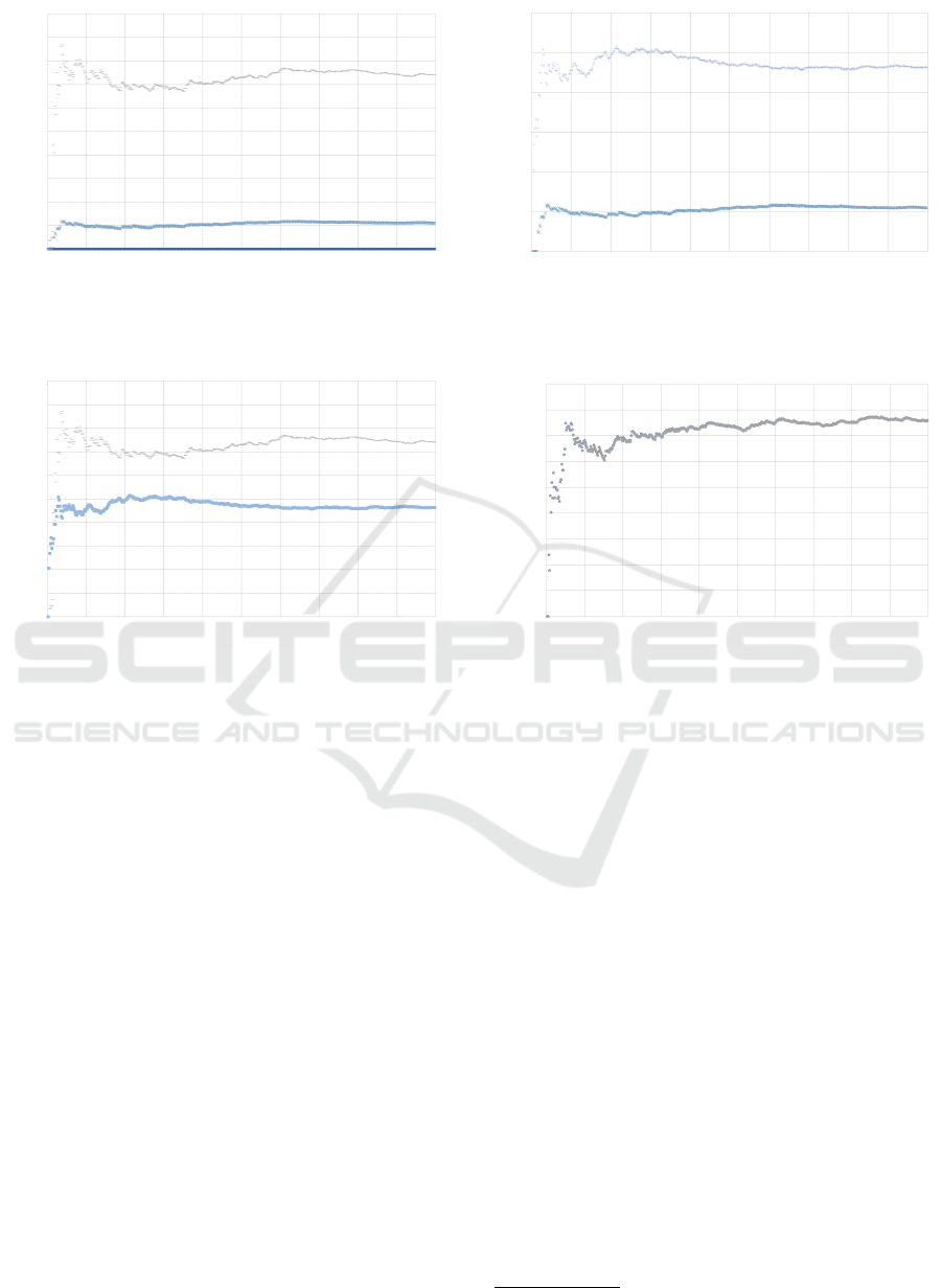
4.3.3 Performance of the Optimization
Algorithms
Finally, we also want to compare how well differ-
ent optimization algorithms perform. We assess the
R functions optim (M
optim
) and nlm (M
nlm
) by repeat-
ing the previous experiment with these two parameter
optimization algorithms.
4.3.4 Error Calculation
Finally, we evaluated which of the two error calcula-
tion approaches e
1
or e
2
is best suited for evaluating
a model with estimated parameters. Error e
1
assumes
that all data is training data, while e
2
divides simi-
lar procedures into training and validation data using
cross-validation.
4.4 Results
4.4.1 One Model and Several Data Sets
The first data set d
1
corresponds well to the model
f
1
. This is the ideal case. As expected, the errors
converge to near zero, cf. Figure 2.
The second data set d
2
is based on a cubic func-
tion, for which a linear model is not a good fit. While
the errors converge, they remain quite large, cf. Fig-
ure 3.
The third data set d
3
is based on a sine function.
The errors converge in this case as well but, are again
relatively high, compared to the first data set, cf. Fig-
ure 4. The reason for this is that a horizontal straight
line can be drawn through the data points, against
which optimization is performed. The data points
are relatively close to each other and the horizontal
straight line.
4.4.2 Several Models and One Data Set
Again, the picture is clear: Although all errors be-
come constant at some point, only the error of the lin-
ear model formula f
1
matching the data points d
1
is
small. The error is a measure of the accuracy of the
model. Figure 5 clearly shows the difference between
a model that fits very well to the data set d
1
and a
model that fits badly to it.
4.4.3 Performance of the Optimization
Algorithms
It shows that there is not a single best algorithm:
while method M
optim
is particularly suitable for f
2
,
cf. Figure 6), method M
nlm
is more suitable for f
3
, cf.
Figure 7. M
optim
and M
nlm
are similarly well suited
Optimization of Software Estimation Models
147


The first set of data points is based on a * x + b and therefore corresponds very well to                   
the model formula. Therefore, the error made is very low and becomes constant. Figure 17              
shows the constellation of the data set, Figure 18 shows how the errors msqe1 und msqe2               
convergetonearzero.Thisisthebestcasewherethemodelfitsverywelltothedatapoints.

Figure17:FirstDataSet
 
34
0 10 20 30 40 50 60
0
50
100
150
200
250
300
350
Figure 1: The first data set with d
1
(x) = A × x + B and a
random seed as generator function.

Figure20:ErrorsofthesecondDataSet 
37
0 50 100 150 200 250 300 350 400 450 500
e
1
e
2
0
2500
5000
7500
10000
12500
Figure 3: Errors for the model on the second data set.
for the trivial case f
1
, cf. Figure 8. So, it makes
sense to provide different optimization algorithms and
to use them in parallel.
4.4.4 Error Calculation
The error calculation uses two approaches e
1
or e
2
.
Figures 2–4 show that their differences are marginal
and converge to zero. However, e
1
is potentially over-
trained and therefore less trustworthy than e
2
.
4.5 Discussion
The evaluation focused on GC 1 and GC 2 and
showed that the model parameters could be trained
from data, are suitable to make predictions, and that
the accuracy improves and converges with the number
of training data points.
The remaining goal criteria are also fulfilled by
the design and do not need to be evaluated experi-
mentally. Since the models are designed by a human
domain expert and only the parameters are optimized,
it can be assumed that they are understandable and
trusted. The parameters that the optimization algo-
rithm determines can easily be validated against the


Figure18:ErrorsofthefirstDataSet

 
35
0.0010
0 50 100 150 200 250 300 350 400 450 500
0
0.0002
0.0004
0.0006
0.0008
e
1
e
2
Figure 2: Errors e
1
and e
2
for the model f
1
(x) = a × x + b
fit to the first data set. Note that the error converge to near
zero and that the two error measures are quite similar.


Figure22:ErrorsofthirdDataSet
If the model formula matches the data points and the error of the model is small, meaningful                
predictions can be made; at least if they are not outliers. For example, in the trivial example,                
the range smaller than 0 and greater than 80 is not modeled because the given data points are                 
not outside this range. However, if the data of a project are for instance 120 or 50, no                 
meaningful prediction can be made. Instead, the system must recognize that it is an outlier              
point.
7.1.2OneSetofDataPoints,MultipleModels
In practice, several models are entered with the same data points. For this reason, in the               
second step of evaluating the three different models were given. This time we vary the              
modelswhilethedatapointsaregeneratedbasedona*x+b.
ThethreeModelsare:
F1:a*x+b
F2:a*x^3+b
39
0 50 100 150 200 250 300 350 400 450 500
0
2
4
6
8
10
12
14
16
e
1
e
2
Figure 4: Errors for the model on the third data set.
data set; hence, GC 5 is fulfilled. Since outliers can
be detected, the error is provided, and the model’s fit
against the data sets can easily be inspected, we con-
sider GC 4 fulfilled as well. The evaluation used ar-
tificial models and synthetic data, with a sample size
of 500 for each data generator, not tied to the soft-
ware estimation domain. While repeating the experi-
ments with real models and data is a matter of future
work, this evaluation method at least shows that the
approach applies to models of different types and do-
mains, so GC 6 is also fulfilled.
GC 3 is fulfilled by the use of PCA to determine
how much explanatory power each parameter has, so
the PCA can suggest that some data points are not
needed for the model. It can also be used to determine
if optional parts of the model should be included or
not based on their explanatory power. This informa-
tion can be provided to the model developer as sug-
gestions.
We can now answer our research questions: Con-
tinuous model improvement can be realized, and new
models can be easily tested and implemented, us-
ing the approach based on optimization algorithms
(RQ1). Data points can be collected while correla-
tions between inputs can be detected by performing
ICSOFT 2019 - 14th International Conference on Software Technologies
148


F3:a*sin(x)+b
7.1.2.1Comparisonofthethreemodels.
First, it should be evaluated which of the three models fits best to the data points. Here again,                 
the picture is clear: Although all errors become constant at some point, only the error of the                
linear model formula matching the data points is small. The error is a measure of the accuracy                
of the model. The following graphic shows very well the difference between a model that fits               
verywelltothedatapointsandamodelthatfitsverybadlytothedatapoints.

Figure23:ComparisonofthreedifferentModels
7.1.2.2Comparisonofthedifferentmethods
The next step is to evaluate which of the two optimization algorithms M1 and M2 is the best.                 
M1usesoptiminR,whileM2usestheRfunctionnlm.
It becomes clear that there is not the best method or the best optimization algorithm. While               
method M1 is particularly suitable for F3 (Figure 26), method M2 is more suitable for F2               
40
0 50 100 150 200 250 300 350 400 450 500
0
1000
2000
3000
4000
5000
6000
7000
8000
9000
10000
f
1
f
2
f
3
Figure 5: Comparison of the models f
1
, f
2
, and f
3
on the
data set generated from d
1
(x) = A × x + B.



Figure25:ComparisonofF1withM1andM2

Figure26:ComparisonofF3withM1andM2
42
0
1000
2000
3000
4000
5000
6000
7000
8000
9000
10000
0 50
100
150 200 250 300
350
400 450
500
M
optim
M
nlm
Figure 7: Comparison of two optimization algorithms,
M
optim
(lower) and M
nlm
(upper) for the model f
3
on the
data set d
1
.
PCA regularly (RQ2). By implementing the proto-
type tool, we showed that the approach could be au-
tomated (RQ3).
5 CONCLUDING REMARKS AND
FUTURE WORK
We suggested an approach to estimation model design
and automated optimization that allows for model
comparison and improvement based on collected data
sets. Our approach simplifies model optimization and
selection. It contributes to a convergence of exist-
ing estimation models to meet contemporary software
technology practices and to a possible selection of the
most appropriate ones.
We evaluated the design and implementation of
our approach and showed that it fulfilled all the goal
criteria that we formulated. The model accuracy is
improved through optimization, and the models are
understandable by human domain experts. We also
find that principal component analysis can determine
the explanatory power of parameters and parts of

(Figure 24). M1 and M2 are similarly well suited for F1 (Figure 25). These facts show that it                 
makessensetousemanydifferentoptimizationalgorithms.

Figure24:ComparisonofF2withM1andM2
41
0 50 100 150 200 250 300 350 400 450 500
0
1000
2000
3000
4000
5000
6000
M
optim
M
nlm
Figure 6: Comparison of two optimization algorithms
M
optim
(lower) and M
nlm
(upper) for the model f
2
on the
data set d
1
.



Figure25:ComparisonofF1withM1andM2

Figure26:ComparisonofF3withM1andM2
42
0 50 100 150 200 250 300 350 400 450 500
0
0.0001
0.0002
0.0003
0.0004
0.0005
0.0006
0.0007
0.0008
0.0009
Figure 8: Comparison of two optimization algorithms,
M
optim
and M
nlm
(overlapping) for the model f
1
on the data
set d
1
.
models can suggest changes to the model developer.
We only evaluated our approach on synthetic data,
so future work is to apply it to data from real-world
software projects. We particularly want to use our ap-
proach to compare models that we design with estab-
lished models such as COCOMO II to see how they
compare. We are also interested to see how the ap-
proach will perform, both concerning accuracy and
performance on larger data sets. Further yet, we re-
lied on a small set of optimization algorithms, and we
plan to incorporate more algorithms, e.g., genetic al-
gorithms in the future.
ACKNOWLEDGMENTS
We are grateful for Andreas Kerren’s valuable feed-
back on the thesis project (Kopetschny, 2018) that this
paper is based on.
The research was supported by The Knowledge
Foundation
2
, within the project “Software technology
for self-adaptive systems” (ref. number 20150088).
2
http://www.kks.se
Optimization of Software Estimation Models
149

REFERENCES
Albrecht, A. (1979). Measuring Application Development
Productivity. In Press, I., editor, IBM Application De-
velopment Symposium, pages 83–92.
Beck, K. and Andres, C. (2004). Extreme Programming
Explained: Embrace Change (2nd Edition). Addison-
Wesley Professional.
Boehm, B. W., Abts, C., Brown, A. W., Chulani, S., Clark,
B. K., Horowitz, E., Madachy, R., Reifer, D. J., and
Steece, B. (2009). Software Cost Estimation with CO-
COMO II. Prentice Hall Press, Upper Saddle River,
NJ, USA, 1st edition edition.
Breunig, M. M., Kriegel, H.-P., Ng, R. T., and Sander, J.
(2000). Lof: Identifying density-based local outliers.
In Proceedings of the 2000 ACM SIGMOD Interna-
tional Conference on Management of Data, SIGMOD
’00, pages 93–104, New York, NY, USA. ACM.
Brooks, Jr., F. P. (1995). The Mythical Man-month (An-
niversary Edition). Addison-Wesley Longman Pub-
lishing Co., Inc., Boston, MA, USA.
Clark, B. (2015). COCOMO
R
 III project purpose.
http://csse.usc.edu/new/wp-content/uploads/2015/04/
COCOMOIII Handout.pdf. Accessed April 12, 2019.
Fletcher, R. (1987). Practical Methods of Optimization;
(2nd Edition). Wiley-Interscience, New York, NY,
USA.
Galorath, D. D. and Evans, M. W. (2006). Software Sizing,
Estimation, and Risk Management. Auerbach Publi-
cations, Boston, MA, USA.
Huang, L. (2017). A quasi-newton algorithm for large-scale
nonlinear equations. Journal of Inequalities and Ap-
plications, 2017(1):35.
Humphrey, W. S. (1996). Using a defined and measured
personal software process. IEEE Software, 13(3):77–
88.
Jenson, R. L. and Bartley, J. W. (1991). Parametric es-
timation of programming effort: An object-oriented
model. Journal of Systems and Software, 15(2):107 –
114.
Karner, G. (1993). Resource estimation for objectory
projects.
Kopetschny, C. (2018). Towards technical value analysis of
software. Master Thesis, 15 HE credits.
Menzies, T., Yang, Y., Mathew, G., Boehm, B., and Hihn, J.
(2017). Negative results for software effort estimation.
Empirical Software Engineering, 22(5):2658–2683.
Nelder, J. A. and Mead, R. (1965). A simplex method
for function minimization. Computer Journal, 7:308–
313.
Office, U. S. (1962). PERT: Program Evaluation Research
Task: Summary Report Phase 1. U.S. Government
Printing Office.
Putnam, L. H. and Myers, W. (1991). Measures for Ex-
cellence: Reliable Software on Time, Within Budget.
Prentice Hall Professional Technical Reference.
Simon, H. A. (1996). The Sciences of the Artificial (3rd
Edition). MIT Press, Cambridge, MA, USA.
Sorensen, D. (1982). Newton’s method with a model trust
region modification. SIAM Journal on Numerical
Analysis, 19(2):409–426.
Spolsky, J. (2007). Evidence based scheduling.
https://www.joelonsoftware.com/2007/10/26/evidence-
based-scheduling/.
Valerdi, R. (2004). Cosysmo working group report. IN-
SIGHT, 7(3):24–25.
ICSOFT 2019 - 14th International Conference on Software Technologies
150