Visual Predictive Control of Robotic Arms with Overlapping Workspace

E. Le Fl

echer

1,2 a

, A. Durand-Petiteville

, V. Cadenat

1,2

and T. Sentenac

CNRS, LAAS, 7 Avenue du Colonel Roche, F-31400 Toulouse, France

Univ. de Toulouse, UPS, F-31400, Toulouse, France

Mechanical Department of Federal University of Pernambuco (UFPE), Recife, Brazil

Keywords:

Agricultural Robotics, Multi-arms, Non-linear Model Predictive Control, Image based Visual Servoing.

Abstract:

This paper deals with multi-arms fruits picking in orchards. More speciﬁcally, the goal is to control the arms

to approach the fruits position. To achieve this task a VPC strategy has been designed to take into account

the dynamic of the environment as well as the various constraints inherent to the mechanical system, visual

servoing manipulation and shared workspace. Our solution has been evaluated in simulation using on PR2

arms model. Different models of visual features prediction have been tested and the entire VPC strategy has

been run on various cases. The obtained results show the interest and the efﬁciency of this strategy to perform

a fruit picking task.

1 INTRODUCTION

To meet the increasing food demands from a grow-

ing world population, agriculture will need to double

its production by 2050. Alternatively, it will need to

reduce its environmental impact to ﬁght against cli-

mate change and avoid to harm soils. Among the so-

lutions presented in (Foley et al., 2011; Grift et al.,

2008), robotics has been designated as one of the most

promising strategies.

Agriculture robotics may operate in various envi-

ronments such as open ﬁelds, orchards, green houses,

... In this work, one focuses on robots perform-

ing weeding, spraying, trimming, or harvesting in

orchards. The autonomous achievement of any of

these tasks requires the same capacities for the robotic

system: (i) autonomously navigate in an orchard;

(ii) detect and localize a set of natural landmarks

of interest; (iii) approach the landmarks with some

robotic manipulators; (iv) manipulate/interact with

the landmarks of interest without damaging them. Af-

ter addressing the autonomous navigation problem in

(Durand-Petiteville et al., 2017; Le Flecher et al.,

2017), the focus is now on the landmark approach

problem when considering a couple of robotic ma-

nipulators embedded on a mobile platform. This

topic has already been addressed during the design

of systems harvesting cucumbers (Van Henten et al.,

https://orcid.org/0000-0002-2683-8675

2003) or tomatoes (Zhao et al., 2016b). Despite

the promising results, the harvesting efﬁciency needs

to be increased to meet the viability demand from

farmers (Zhao et al., 2016a). To do so, one of the

most adopted approach consists of embedding several

robotics arms on the mobile platform, as it is done

in (Zhao et al., 2016a) for a melon harvester. How-

ever, it is pointed in (Vougioukas et al., 2016) that

fruits are not uniformly distributed on commercial or-

chards trees. Indeed, to maximize the fruits accessi-

bility, growers use speciﬁc trees with high fruits den-

sity, thus facilitating the manual harvesting. For this

reason, during the design of a harvesting system, it

seems then interesting to consider the use of several

arms whose workspace overlap. Thus, even if the

arms do not collaborate to manipulate one single ob-

ject, they share a common workspace. It is then possi-

ble to use several arms to pick fruits in the same high

density area, which decreases the overall harvesting

time.

Regarding the control of the robotics arms, it

seems interesting to focus on reactive controllers.

Thus, when considering the harvesting problem, a tree

is a highly dynamic environment because of the ﬂex-

ibility of the branches and the weight of the fruits:

each time a fruit is harvested, the local distribution of

fruits and branches is modiﬁed. It is then proposed

to use an image based visual servoing (IBVS) scheme

for its reactive capabilities (Chaumette and Hutchin-

son, 2006). This kind of controller will track the fruit

130

Flécher, E., Durand-Petiteville, A., Cadenat, V. and Sentenac, T.

Visual Predictive Control of Robotic Arms with Overlapping Workspace.

DOI: 10.5220/0008119001300137

In Proceedings of the 16th International Conference on Informatics in Control, Automation and Robotics (ICINCO 2019), pages 130-137

ISBN: 978-989-758-380-3

of interest and use its coordinates in the image to con-

trol the arm. However, IBVS schemes working in the

image space, they do not provide any guarantee re-

garding the trajectory of the camera in the workspace.

This represents a major issue when considering arms

sharing a common workspace. A well adopted solu-

tion to take into account constraints on position, ve-

locity, or workspace is the model predictive control

scheme. Indeed, when minimizing the cost function,

the solver can deal with numerous constraints (Diehl

and Mombaur, 2006). Thus, to obtain a reactive con-

troller dealing with constraints, it is proposed to de-

sign an IBVS-based NMPC (nonlinear model predic-

tive control) controller, also named Visual Predictive

Control (VPC). For this particular case, the cost func-

tion is deﬁned as the error between the image coordi-

nates of the visual features representing the landmark

of interest at the current pose and the desired one.

Similar control schemes have been already pro-

posed. For example, in (Allibert et al., 2010) several

prediction models are used to simulate the control of

a 6 DOF camera subject to visibility constraints. In

(Sauvee et al., 2006), the designed controller deals

with torques, joints and image constraints and is eval-

uated in simulations. In (Hajiloo et al., 2015) an

IBVS-based MPC controller using a tensor product

model is developed. It also takes into account actua-

tors limitations and visibility constraints.

In this paper, it is proposed to extend the VPC

case to the control of two arms sharing a common

workspace. Thus, in addition to drive the two end-

effectors to their desired pose using the image space,

the controllers have to guarantee the non-collision be-

tween both arms.

A non-linear predictive control strategy to perform

a reactive control based on IBVS method is simulated

on a robot equipped of multiple arms with eye-in-

hand cameras. Each arm needs to achieve separate

tasks sharing the same workspace. These tasks are

subject to constraints such as the restricted ﬁeld of

view, the kinematic (joints limits in position and ve-

locity) but also the self collision constraints.

The paper is organized as follows. In section II

the robot model to estimate the location of visual fea-

tures is deﬁned. In section III, the control strategy is

explained, as well as the cost function described and

the diverse constraints designed. Section IV is dedi-

cated to the simulation results obtained while section

V summarizes and develops the expectations for the

future.

2 MODELING

In this section, one ﬁrst focuses on the modeling of

the system, i.e., the robotic arms, the cameras and the

targets. Then, two models to predict the visual feature

coordinates of a point are presented. One ends with a

discussion regarding the viability of these models for

the visual predictive control problem.

2.1 System Modeling

The robotic system considered in this work is com-

posed of n

identical arms, each of them contain-

ing m

revolute joints. A camera is attached to the

end effector of each arm. To model, the system,

let us ﬁrst deﬁne a global frame F

= (O

)

attached to the system base. Moreover, n

frames

= (O

), with i ∈ [1, ...,n

], are used to

represent the pose of the camera attached to the i

arm.

One denotes q

i j

and ˙q

i j

, with j ∈ [1,...,m

respectively the angular position and velocity of

the j

joint of the i

arm. Thus, for the i

arm, one obtains the conﬁguration vector Q

,...,q

]

and the control input vector

[ ˙q

, ˙q

,..., ˙q

]

. Finally, we deﬁne for the whole

system Q = [Q

,...,Q

]

and

Q = [

,...,

]

The cameras mounted on the end effectors are

modeled using the pinhole model. Thus, the pro-

jection matrices H

mapping the 3D coordinates

(x,y,z) of a point in the camera frame F

to its 2D

projection (X,Y ) on the image plan F

is deﬁned as

follows:



















f /z 0 0 0

0 f /z 0 0

0 0 1 0

0 0 0 1



















(1)

In this work, the arms are controlled to make each

camera reach a pose deﬁned by the coordinates of

point visual features in the image space. To do so, one

uses n

landmarks made of four points. When consid-

ering the i

camera/target couple, the coordinates of

the projection of each point on the image is denoted

= [X

]

, with i ∈ [1,...,n

] and l ∈ [1, 2,3,4].

Thus, the visual feature vector for each camera is de-

ﬁned as S

= [S

]

, whereas the system

one is given by S = [S

,...,S

]

. In the same way,

a vector for the visual feature desired coordinates of

each camera is deﬁned as S

∗

= [S

∗

]

Visual Predictive Control of Robotic Arms with Overlapping Workspace

131

2.2 Prediction Models

A visual predictive control scheme requires to be able

to predict the values of the visual features for a given

sequence of control inputs. In (Allibert et al., 2010),

the authors present two ways to perform the predic-

tion step for a ﬂying camera: the local and global ap-

proaches. This section is devoted to the presentation

of both methods for the case of a 6 degrees of freedom

camera embedded on a robotic arm.

2.2.1 The Global Model

The global approach is based on the robot geomet-

ric model and the camera projection matrix. The idea

consists of computing the 3D coordinates of the fea-

tures in the next camera frame, then to project them

onto the camera image plan. To do so, let us con-

sider a discrete time system with a sampling period

, where t

k+1

= t

+ T

, and the notation .(k) = .(t

The conﬁguration Q

(k + 1) of the i

arm, with i ∈

[1,...,n

], at the next iteration obtained after applying

the control inputs

(k) is given by:

(k +1) = Q

(k) +

(k)T

(2)

Knowing the arm conﬁguration at instants t

and t

k+1

it is then possible to compute the homogeneous trans-

formation matrices between the camera frame F

and

the base one F

¯o

(.) = H

b/c

(.) ¯o

(.) (3)

where ¯o are the homogeneous coordinates of a point

feature expressed in the base or camera frame. Fi-

nally, coupling (3) with (1), one obtains a predic-

tion of the coordinates of a point feature in the image

space.

(k +1) =

(k +1)H

−1

b/c

(k +1)H

b/c

(k)H

−1

(k)S

(k)

(4)

2.2.2 The Local Model

The local approach relies on the differential equation

mapping the derivative of the visual feature coordi-

nates

to the robot control input vector

. To ob-

tain this equation, one uses the robot’s Jacobian J

mapping the camera kinematic screw T

and

(5),

and the interaction matrix L

, mapping

to T

(6).

= J

(5)

= L

(6)

where

−

−(1 + X

) Y

0 −

1 +Y

−X

(7)

By combining equations (5) and (6), one obtains the

following local model for each arm/camera couple:

= L

(8)

2.2.3 Usability of the Models

When considering using one of the models on an ex-

perimental system, several aspects have to be taken

into account. First, both models require a mea-

sure/estimate of the visual feature depth z (see equa-

tions (1) and (7)). However, when using a monocular

camera, this value can only be retrieved by estimation.

Another widely adopted option, consists of using a

constant value, such as the depth value at the initial

or desired pose (Chaumette and Hutchinson, 2006).

The second issue is related to the integration of the

local model to obtain the prediction equation. A ﬁrst

option consists of using an advanced numeric scheme

to accurately compute the integration, whereas a sec-

ond one relies on a linear approximation of the model,

such as:

(k +1) = S

(k) +L

(k)T

(9)

Thus, depending on the user choices regarding these

issues, the prediction feature coordinates will be more

or less accurate. In section 4, different conﬁgurations

will be evaluated for our speciﬁc application in order

to select the most appropriate and realistic solution.

3 CONTROLLER DESIGN

In this section the control of the arms motion to reach

their own targets and compounding necessary con-

straints are presented. To achieve these goals, NMPC

control has been implemented to ﬁnd the optimal in-

puts vector which minimizes a cost function subjects

to constraints. To do so, we ﬁrst present the cost func-

tion to be minimized in order to reach the desired tar-

gets. Then, the expression of each constraint will be

deﬁned.

3.1 Visual Predictive Control

The proposed VPC scheme couples NMPC (Nonlin-

ear Model Predictive Control) with IBVS (Image-

Based Visual Servoing). Thus, similarly to NMPC,

it consists of computing an optimal control sequence

Q(.) that minimizes a cost function J

over a pre-

diction horizon of N

steps while taking into account

a set of user-deﬁned constraints C(

Q(.)). Moreover,

similarly to IBVS, the task to achieve is deﬁned as an

error in the image space. Thus, the cost function to

ICINCO 2019 - 16th International Conference on Informatics in Control, Automation and Robotics

132

minimize is the sum of the quadratic error between

the visual feature coordinates

S(.) predicted over the

horizon N

and the desired ones S

∗

. It then possible

to write the VPC problem as:

Q(.) = min

Q(.)



(S(k),

Q(.))



(10)

with

(S(k),

Q(.)) =

k+N

−1

∑

p=k+1

[

S(p) − S

∗

]

[

S(p) − S

∗

]

(11)

subject to

S(.) = (4) or (8) (12a)

S(k) = S(k) (12b)

Q(.)) ≤ 0 (12c)

As mentioned in the previous section, the visual fea-

ture coordinates can be predicted either using the

global or local models (equation (12a)). To compute

the prediction, one uses the last measured visual fea-

tures (equation (12b)). Finally, equation (12c) deﬁnes

the set of constraints to be taken into account when

minimizing the cost function (11).

Thus, solving equation (10) leads to the optimal

sequence of control inputs

Q(.). In this work, and

as it is usually done, only the ﬁrst element

Q(1) of

the sequence is applied to the system. At the next

iteration, the minimization problem is restarted, and a

new sequence of optimal control inputs is computed.

This loop is repeated until the task is achieved, e.i.,

the cost function (11) is vanished.

3.2 Constraints

As seen in the previous section, it is possible to add a

set of constraints in the minimization problem. In this

section, one presents the constraints related to the ge-

ometry of the robot, the velocity of the joints, and the

ﬁeld of view of the camera. One ﬁnishes with deﬁning

a set of constraints that guarantee the non-collision of

the arms despite sharing a common workspace.

3.2.1 System Constraints

The joint velocity lower and upper bounds are respec-

tively denoted

min

and

max

. They are two N

long

vector, with N

= n

. They allow to deﬁne the

lower and upper limit of each joint of each arm over

the prediction horizon. Consequently, the constraint

Q(.) is described in the domain κ = [

min

max

and the velocity constraint is then written as:



Q −

max

min

−



≤ 0 (13)

Mechanical limits follow the same principle. The

lower and upper bounds of the angular values are de-

noted Q

min

and Q

max

. They are two N

long vector,

with N

= n

. These constraints are then given

by:



Q − Q

max

min

− Q



≤ 0 (14)

Finally, the visual constraints are deﬁned by the

image dimension. Ones denotes the bounds by S

min

and S

max

. They are two N

long vector, with N

. Thus, all the predicted visual features coor-

dinates need to be kept into this space, and the con-

straints can then be written as:



S − S

max

min

− S



≤ 0 (15)

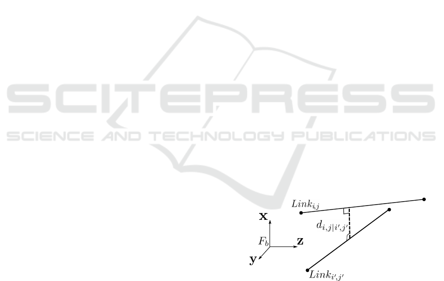
3.2.2 Overlapping Workspace Constraint

Due to the overlapping workspace, it is mandatory

to guarantee the non-collision between the arms. To

do so, one computes the shortest distance d

i, j|i

, j

be-

tween the j

joint of the i

arm and the j

0th

joint of

the i

0th

arm. The closest distance is evaluated as the

norm of the segment perpendicular to both assessed

links as it is illustrated in ﬁgure 1. Finally, in order to

avoid collision, one deﬁnes the following constraint:



min

− d



≤ 0 (16)

where d = [d

1,1|2,1

,...,d

−1,m

] and d

min

is a pre-

deﬁned distance.

Figure 1: Computation of the shortest distance d

i, j|i

, j

be-

tween links L

i j

and L

3.2.3 Terminal Constraint

To make the system converge, it is mandatory to guar-

antee that the predictive control problem is feasible

(Lars and Pannek, 2016). To check the feasability, one

adds a ﬁnal constraint in the optimization problem. It

is deﬁned as the error between the prediction of the vi-

sual feature coordinates

S(k + N

− 1) obtained at the

Visual Predictive Control of Robotic Arms with Overlapping Workspace

133

end of the prediction horizon, and the desired ones S

∗

If the solver cannot compute a sequence of control in-

puts

Q that respects this constraint, then the problem

is not feasible, and there is no guarantee regarding the

system convergence.



S(k + N

− 1) − S

∗



≤ 0 (17)

All the constraints are now deﬁned and can be in-

tegrated into the non-linear function C(

Q(.)):

Q) ≤ 0 ⇒







Q −

max

min

−

Q − Q

max

min

− Q

S − S

max

min

− S

min

− D

S(k + N

− 1) − S

∗







≤ 0 (18)

Thus, the optimal input must belong to the domain

deﬁned by C(

Q(.)).

4 SIMULATION

In this section, one presents the results obtained by

simulating the control of two arms with MATLAB

software. A 7 DOF model has been selected, based on

the arms embedded on the PR2 robot. In these simu-

lations the task consists of positioning the cameras at-

tached to each end-effector with respect to two given

targets. Each desired position is deﬁned in the image

space by S

= [x

], which are

the coordinates of four points representing the corre-

sponding target. Moreover, the prediction horizon is

set up at N

= 5. Regarding the constraints, the an-

gular velocity limits for the ﬁrst prediction step are

given by κ = [−0.2 0.2] for each joint, whereas it

is extended to κ = [−5 5] for the rest of the predic-

tion step. This allows to decrease the computation

while guaranteeing a feasible control input for the

ﬁrst step. The size of the image is S

min

= [−4 − 4]

and S

max

= [4 4]. The angular constraints on each

joint are setup as described in the PR2 documenta-

tion (Garage, 2012). Finally the minimum collision

avoidance distance is ﬁxed to D

min

= 0.1. The ini-

tial coordinate of the visual features are computed

based on the initial conﬁguration of the robot given

by q

init

= [0

0 0 0 0 0 0

0 0 0 0 0]

for every

simulation. Finally, one ﬁxes T

= 50ms.

4.1 Comparison between Different

Prediction Methods

The ﬁrst set of simulation assesses the accuracy of

different predictive models presented in section 2.2.

To do so, one drives the arms from q

init

to q

∗

[−

0 0 0 0 0 0

0 0 0 0 0]

. During this motion,

the coordinates of the visual features predicted over

the prediction horizon, are compared with a ground

truth. In this case, it consists of the prediction ob-

tained with the global model computed with the real

depth of each visual feature.

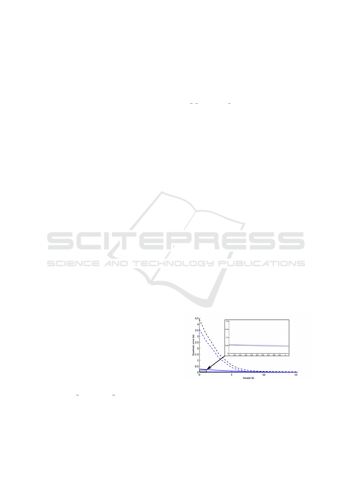
Figure 2 shows the evolution over the simulation

of the quadratic error between the predicted coordi-

nates of one visual feature and the ground truth. Six

models are compared by combining the global model

(solid lines), local Euler approximation (dashed lines)

and local Runge Kutta approximation (dotted lines)

with the depth values real z (black) and desired z

∗

(blue). It can be seen that the global models and

the local Runge Kutta are signiﬁcantly more accu-

rate than the local Euler one. Indeed, using this latter

prediction scheme introduces a large error, and might

not allow the system to converge toward the desired

conﬁguration. In a second ﬁgure 3, the previous er-

rors were summed over the simulation to offer a bet-

ter view of model performances. When considering

the use of the real depth, the global model is the most

accurate. However, this result is obtained in a sim-

ulation, and its use in a real context would require

an estimator of the depth. Thus, one now considers

one more realistic case where the depth is approxi-

mated with the constant value z

∗

. In this case, the

local Runge Kutta is the most accurate model. Thus,

for the rest of the simulations the local Runge Kutta

model with z

∗

is used to evaluate the performances in

a more realistic scenario.

Figure 2: Quadratic errors of prediction over the simulation

-Solid: Global model -Dashed: Local Euler -Dotted: Local

Runge Kutta -Black: Real z -Blue: Desired z.

ICINCO 2019 - 16th International Conference on Informatics in Control, Automation and Robotics

134

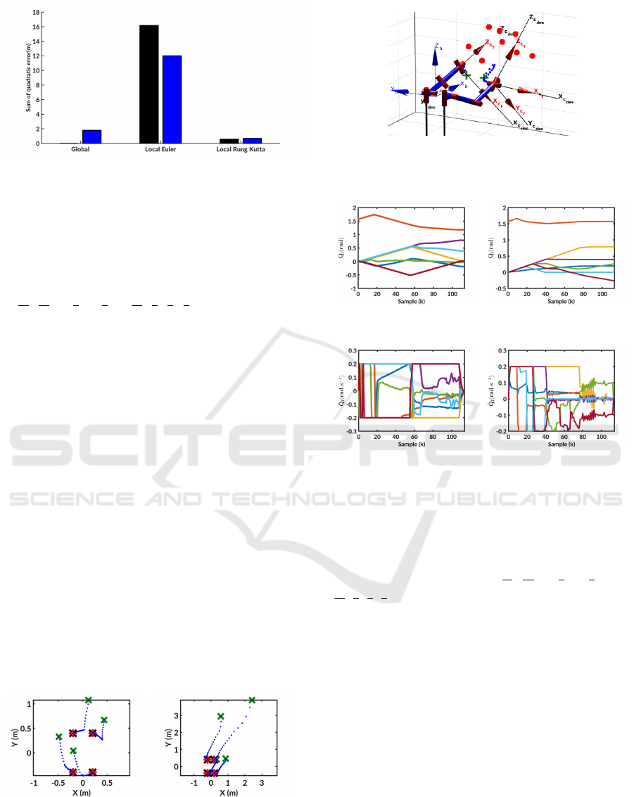
Figure 3: Sum of the quadratic errors of prediction for

global, local Euler and local Runge-Kutta methods -Black:

Real z -Blue: Desired z.

4.2 First Validation

For the second simulation, the system has

to reach the desired conﬁguration q

∗

[−

3π

0 0 0]

from the

initial one q

init

while dealing with the previously

presented constraints. This visual predictive control

was performed using the local model with Runge

Kutta approximation and the desired depth z

∗

. The

trajectories in the images of visual features are

displayed in ﬁgure 4 and show the achievement of

the task for both cameras. Indeed, the proposed

controller was able to drive both arms to make the

cameras converge towards the desired features from

the initial ones (respectively represented by the

red and green crosses in ﬁgures 4(a) and 4(b)). To

achieve the task in the image space, the arms had

to reach the poses presented in ﬁgure 5. During the

realization of this task, the image limits were never

reached. Similarly there was no risk of collision

during the servoing. Moreover, it can be seen in

ﬁgures 6(a) and 6(b) that the constraints on the joint

conﬁgurations were taken into account. Similarly, in

ﬁgures 6(c) and 6(d), one can see that the constraints

on the joint velocities were taken into account to

achieve the task. Indeed, the applied commands stay

within the given range κ = [−0.2 0.2] all along the

simulation.

(a) Left camera - Local

model

(b) Right camera - Local

model

Figure 4: Visual features location using local Runge-Kutta

model and real z - Blue dotted: Trajectories - Red crosses:

Final locations - Green crosses: Initial locations.

Figure 5: Final poses of the arms - Red dots represent the

two targets - Green crosses are the initial poses of the end

effectors.

(a) Right arm joints angular

values

(b) Left arm joints angular

values

velocities

(d) Left arm joints angular

velocities

Figure 6: Joint conﬁgurations and velocities.

4.3 Collision Avoidance

In this last simulation, the system has to reach the

desired conﬁguration q

∗

= [

3π

0 −

0 0 0]

. This set is run using the Runge

Kutta local model with the desired depth values. One

more time the desired visual features are reached from

the initial poses (ﬁgure 7). However, as it can be seen

in ﬁgure 8, the arms had to cross each other to reach

the desired poses. Thanks to the shared environment

constraint included in the control problem, the colli-

sion was avoided. Indeed, ﬁgure 9 shows that the dis-

tance between the different links was never smaller

than the ﬁxed value D

min

= 0.1. In addition, the con-

straints on the joints angular values are respected. In

ﬁgure 10, it can be seen that the right arm joints never

reach their angular limits represented by red dashed

lines (the joints represented in ﬁgures 10(e) and 10(g)

do not have limits on PR2 robot). Similarly, the con-

trol inputs of the right arm present saturations due to

the angular velocity constraints, represented by red

dashed lines in ﬁgure 11, but never goes beyond.

Visual Predictive Control of Robotic Arms with Overlapping Workspace

135

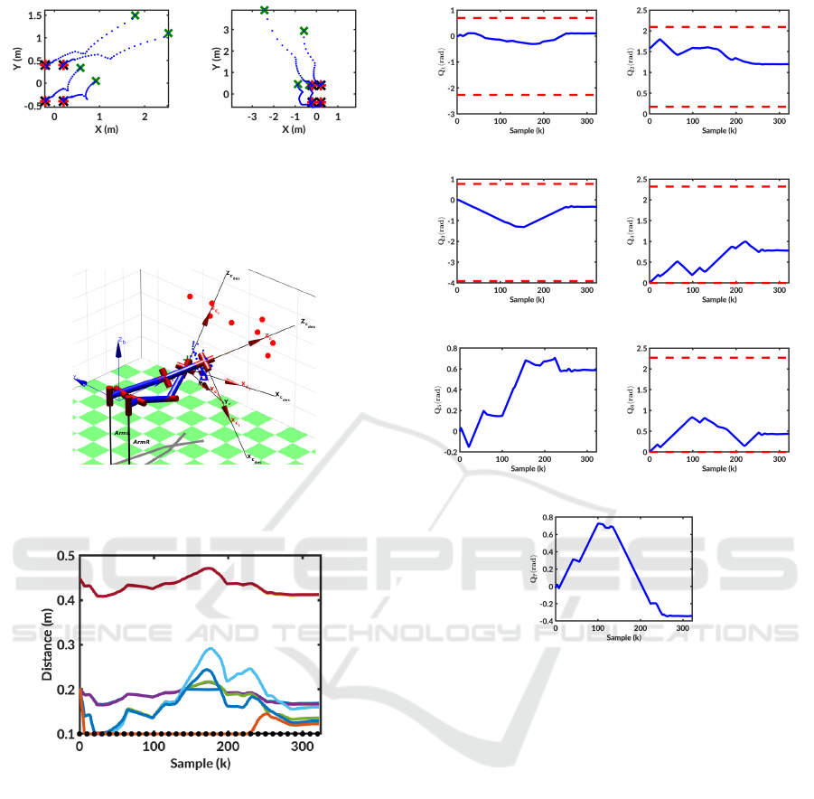
(a) Visual features in image

left

(b) Visual features in image

right

Figure 7: Visual features location using local Runge-Kutta

model and real z - Blue dotted: Trajectories - Red crosses:

Final locations - Green crosses: Initial locations.

Figure 8: Final poses of the arms - Red dots represent the

two targets - Green crosses are the initial poses of the end

effectors.

Figure 9: Collision distance d - Solid: Distances between

links, Dotted: Minimal allowed distance.

5 CONCLUSION

In this paper, we have addressed the problem of fruit

picking in orchards performed by a multi-arms robot.

The goal is to bring the different end-effectors close

to their designated fruits while taking into account the

dynamic environment as well as the constraints in-

herent to the system mechanics, the visual manipu-

lation and the shared workspace. The proposed solu-

tion relies on a VPC strategy to fulﬁll these require-

ments. First, several prediction models were pre-

sented. Next, the visual servoing task and the con-

straints were described including them in a NMPC

(a) q

joint angular values (b) q

joint angular values

joint angular values (d) q

joint angular values

(e) q

joint angular values (f) q

joint angular values

(g) q

joint angular values

Figure 10: Conﬁguration of the right arm over the simu-

lation - Blue solid: Angular joint value q

1 j

- Red dashed:

Maximum angles.

strategy. Finally, simulations based on PR2 manip-

ulators were performed to assess the performance of

each predictive model and to validate the completion

of the servoing. The obtained results show the efﬁ-

ciency of this approach to perform various tasks in a

shared workspace. However, multiple steps still need

to be accomplished. First, this method must be inte-

grated on a real robot. This step will require to opti-

mize the computational time to run it in real time. In

addition, a constraint avoiding the target occlusions

in the image must be integrated. Finally, this manip-

ulation controller will be coupled with our previous

works about the autonomous navigation in orchards

to perform a complete fruits picking task.

ICINCO 2019 - 16th International Conference on Informatics in Control, Automation and Robotics

136

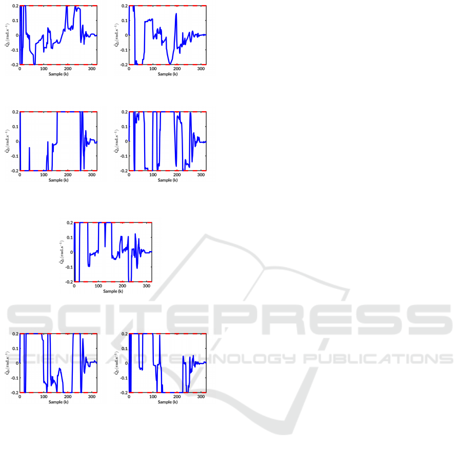
(a) ˙q

joints angular veloc-

ity

(b) ˙q

joints angular veloc-

ity

joints angular veloc-

ity

(d) ˙q

joints angular veloc-

ity

(e) ˙q

joints angular veloc-

ity

(f) ˙q

joints angular veloc-

ity

(g) ˙q

joints angular veloc-

ity

Figure 11: Right arm joints velocities - Blue solid: Joint

velocity value - Red dashed: Maximum velocities.

REFERENCES

Allibert, G., Courtial, E., and Chaumette, F. (2010). Pre-

dictive Control for Constrained Image-Based Visual

Servoing. IEEE Transactions on Robotics, 26(5):933–

939.

Chaumette, F. and Hutchinson, S. (2006). Visual servo con-

trol. i. basic approaches. IEEE Robotics & Automation

Magazine, 13(4):82–90.

Diehl, M. and Mombaur, K., editors (2006). Fast motions

in biomechanics and robotics: optimization and feed-

back control. Number 340 in Lecture notes in con-

trol and information sciences. Springer, Berlin ; New

York. OCLC: ocm71814232.

Durand-Petiteville, A., Le Flecher, E., Cadenat, V., Sen-

tenac, T., and Vougioukas, S. (2017). Design of a

sensor-based controller performing u-turn to navigate

in orchards. In Proc. Int. Conf. Inform. Control, Au-

tomat. Robot., volume 2, pages 172–181.

Foley, J. A., Ramankutty, N., Brauman, K. A., Cassidy,

E. S., Gerber, J. S., Johnston, M., Mueller, N. D.,

O’Connell, C., Ray, D. K., West, P. C., Balzer, C.,

Bennett, E. M., Carpenter, S. R., Hill, J., Monfreda,

C., Polasky, S., Rockstr

om, J., Sheehan, J., Siebert,

S., Tilman, D., and Zaks, D. P. M. (2011). Solutions

for a cultivated planet. Nature, 478:337–342.

Garage, W. (2012). Pr2 user manual.

Grift, T., Zhang, Q., Kondo, N., and Ting, K. C. (2008). A

review of automation and robotics for the bio- indus-

try. Journal of Biomechatronics Engineering, 1(1):19.

Hajiloo, A., Keshmiri, M., Xie, W.-F., and Wang, T.-T.

(2015). Robust On-Line Model Predictive Control for

a Constrained Image Based Visual Servoing. IEEE

Transactions on Industrial Electronics, pages 1–1.

Lars, G. and Pannek, J. (2016). Nonlinear model predictive

control. Springer Berlin Heidelberg, New York, NY.

Le Flecher, E., Durand-Petiteville, A., Cadenat, V., Sen-

tenac, T., and Vougioukas, S. (2017). Implementa-

tion on a harvesting robot of a sensor-based controller

performing a u-turn. In 2017 IEEE International

Workshop of Electronics, Control, Measurement, Sig-

nals and their Application to Mechatronics (ECMSM),

pages 1–6. IEEE.

Sauvee, M., Poignet, P., Dombre, E., and Courtial, E.

(2006). Image Based Visual Servoing through Non-

linear Model Predictive Control. In Proceedings of

the 45th IEEE Conference on Decision and Control,

pages 1776–1781, San Diego, CA, USA. IEEE.

Van Henten, E., Hemming, J., Van Tuijl, B., Kornet, J., and

Bontsema, J. (2003). Collision-free Motion Planning

for a Cucumber Picking Robot. Biosystems Engineer-

ing, 86(2):135–144.

Vougioukas, S. G., Arikapudi, R., and Munic, J.

(2016). A Study of Fruit Reachability in Orchard

Trees by Linear-Only Motion. IFAC-PapersOnLine,

49(16):277–280.

Zhao, Y., Gong, L., Huang, Y., and Liu, C. (2016a). A

review of key techniques of vision-based control for

harvesting robot. Computers and Electronics in Agri-

culture, 127:311–323.

Zhao, Y., Gong, L., Liu, C., and Huang, Y. (2016b). Dual-

arm Robot Design and Testing for Harvesting Tomato

in Greenhouse. IFAC-PapersOnLine, 49(16):161–

165.

Visual Predictive Control of Robotic Arms with Overlapping Workspace

137