Explorations and Lessons Learned in Building an Autonomous Formula
SAE
a
Car from Simulations
Dean Zadok
b,1
, Tom Hirshberg
b,1
, Amir Biran
1
, Kira Radinsky
1
and Ashish Kapoor
2
1
Computer Science Department, Technion, Haifa, Israel
2
Microsoft Research, Redmond, WA, U.S.A.
Keywords:
Autonomous Driving, Imitation Learning, Deep Neural Networks.
Abstract:
This paper describes the exploration and learnings during the process of developing a self-driving algorithm
in simulation, followed by deployment on a real car. We specifically concentrate on the Formula Student
Driverless competition. In such competitions, a formula race car, designed and built by students, is challenged
to drive through previously unseen tracks that are marked by traffic cones. We explore and highlight the
challenges associated with training a deep neural network that uses a single camera as input for inferring car
steering angles in real-time. The paper explores in-depth creation of simulation, usage of simulations to train
and validate the software stack and then finally the engineering challenges associated with the deployment of
the system in real-world.
1 INTRODUCTION
Machine Learning (ML) paradigms such as su-
pervised learning, imitation learning, learning-by-
demonstration and transfer learning are significantly
transforming the field of robotics. However, training a
real-world robot is quite challenging due to high sam-
ple complexity of these methods - successful training
of deep Neural Networks require millions of exam-
ples. The primary means to solve this problem has
been to train models in simulation and then deploy
them in the real world. There are various challenges
with such a workflow (Tan et al., 2018; Peng et al.,
2017) and this paper explores these issues by creating
a real-world autonomous car that was trained com-
pletely end-to-end in a simulation.
In particular, the objective of this work was to
create an autonomous formula student car that could
compete in an international self-driving formula stu-
dent competition in Germany. The competition takes
place on a professional Formula racetrack. Two lines
of traffic cones (blue and yellow cones) define the
track. Note that the track is unknown prior to the race,
so the goal was to create an autonomous system that
could maneuver around accurately on arbitrary and
a
A student formula design competition organized by
SAE International (previously known as the Society of Au-
tomotive Engineers).
b
The authors contributed equally to this work.
Input DNN Controller
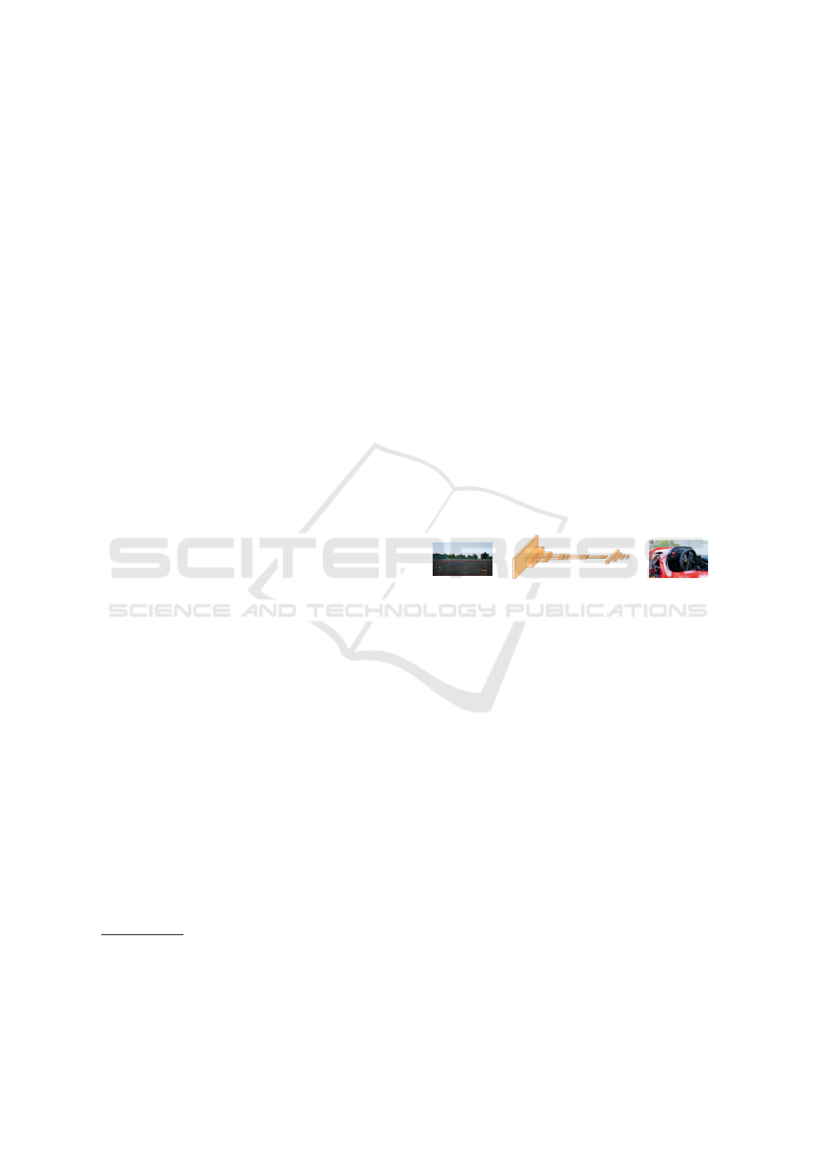
Figure 1: End-to-end deep learning approach. The con-
troller acts according to a predicted steering angle from the
trained DNN. The predicted steering angle is inferred from
a region of interest of a given image. This methodology is
applied both in simulation, and in real-world environments.
unfamiliar tracks. Further, the race scene could po-
tentially include ad signs, tires, grandstands, fences,
etc.
There are several challenges associated with de-
signing and implementing such a system. First, creat-
ing a test environment in order to engineer such a sys-
tem is not only cumbersome and expensive, but also
quite complex due to safety considerations. Secondly,
building an end-to-end system requires several com-
plex engineered systems, both in hardware and soft-
ware, to work together - often such integrations are
challenging, and such dependencies can greatly im-
pede rapid development of individual systems (e.g.,
progress on autonomous software stack crucially de-
pends upon bug-free hardware). Finally, much of the
recent autonomous system modules depend upon the
ability to collect a large amount of training data. Such
data collection is not scalable in real-world due to
both the complexity as well as resource requirements
414
Zadok, D., Hirshberg, T., Biran, A., Radinsky, K. and Kapoor, A.
Explorations and Lessons Learned in Building an Autonomous Formula SAE Car from Simulations.
DOI: 10.5220/0008120604140421
In Proceedings of the 9th International Conference on Simulation and Modeling Methodologies, Technologies and Applications (SIMULTECH 2019), pages 414-421
ISBN: 978-989-758-381-0
Copyright
c
2019 by SCITEPRESS – Science and Technology Publications, Lda. All rights reserved
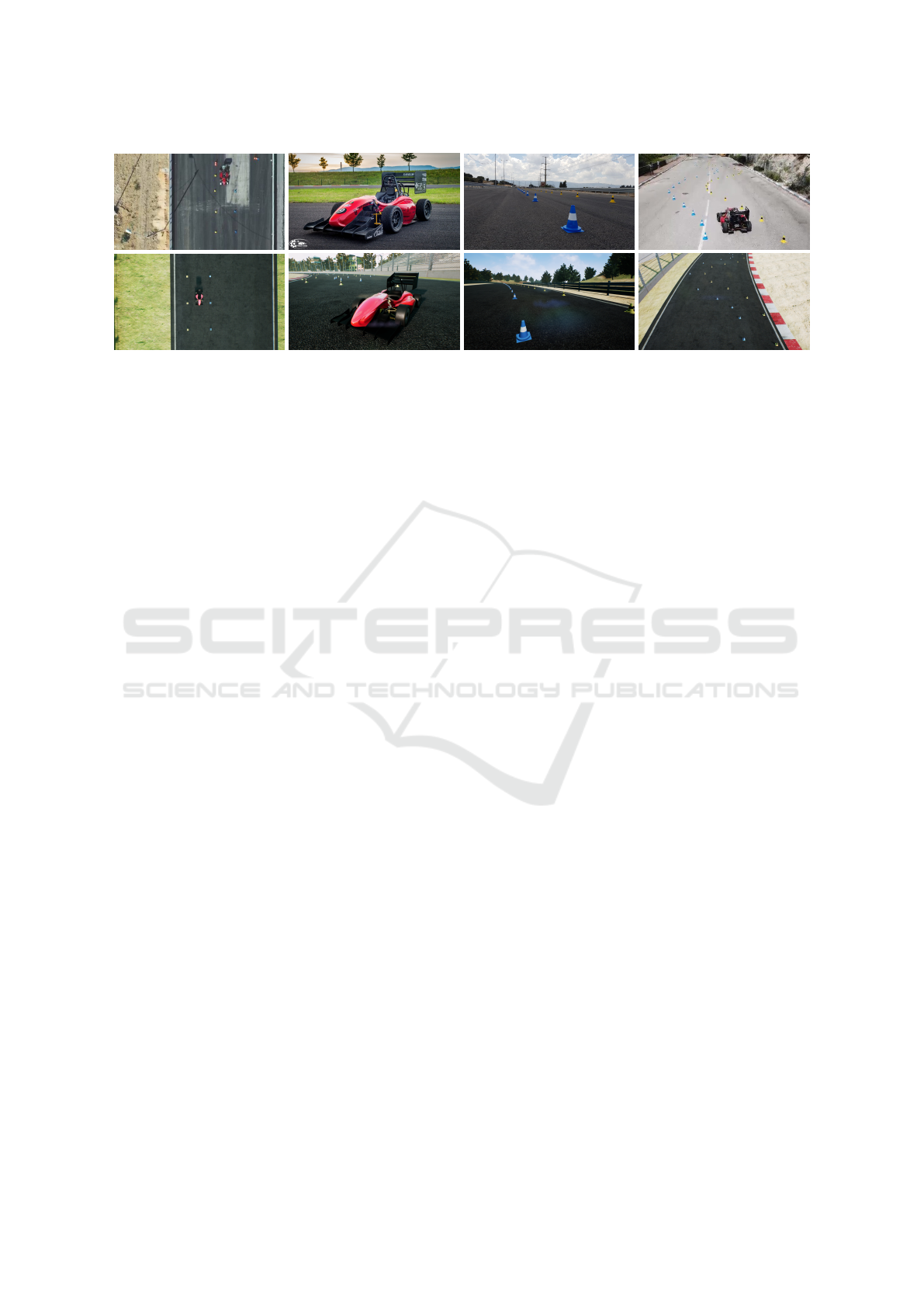
Figure 2: Images taken from our simulated environment (bottom) and from real tracks we have driven in (top). The simulation
was built to have objects resemble their real-world counterparts precisely, including the exact traffic cones and our Formula
SAE car. Both the real world and the simulated environments consisted of straight and swerved tracks as shown. Our model
was trained in simulation only and was executed in a real-world environment.
to carry out such training missions.
We alleviated these problems by training and val-
idating our autonomous stack in simulation. Such
simulations allow us to mitigate risks associated with
safety, enable us to bypass the need to access a closed
off-road track and minimize the dependency on the
development of the hardware stack. Most impor-
tantly, such simulations allow us to gather data at
scale, in a wide variety of conditions, which is not fea-
sible in real-world. Our simulations consist of a dy-
namic model of the custom car, a variety of racetrack
scenes and synthesis of different weather conditions.
We explore and demonstrate that such simulations can
indeed be very useful in building autonomous systems
that are deployed in real-world. We especially high-
light the importance of creating high-fidelity scenes
that mimic the real-environment. We also aim to build
our models completely in simulation, without requir-
ing the system ever to see the real tracks.
At the heart of the system is a Deep Neural Net-
work (DNN) which is trained via imitation learning
(Codevilla et al., 2018). The main task of the DNN is
to predict the desired set of actions the car should take
in real time, given the state the car was in relative to
the environment. The DNN was trained to imitate the
actions of test subjects who first drove the car around
in the simulation during the training data collection
phase. We also investigate challenges associated with
deploying such a trained model on a real car. Specif-
ically, transferring the trained model from simulation
to the real-world consisted of creating a computation-
ally efficient deployment on an edge device that could
result in a high frame-rate, for real-time predictive
performance. This part of our work required vari-
ous optimizations from software engineering includ-
ing the ability to operate using low-power systems. In
summary, various contributions of this paper include:
• An end-to-end design and deployment of an au-
tonomous stack that can drive a custom Formula
SAE car.
• Unique augmentations that alleviate the recording
procedure and improve the trained model substan-
tially.
• A detailed overview of how such predictive sys-
tems trained in simulations can be deployed on a
system that operates in a real-world environment.
The implementation is available at the repository
https://github.com/FSTDriverless/AirSim.
2 RELATED WORK
The industry of autonomous driving has seen a lot of
changes over the past few years. The improvements
in computer vision applications using deep learning
tools had encouraged teams to turn to modern meth-
ods rather than using classic algorithms, or to have
incorporated these new technologies in hybrid-type
approaches. The DARPA competition, initiated in
2004, served as a ground for teams to advance au-
tonomous technologies in a significant manner. Such
team describes in (Urmson et al., 2008) the vehicle
that had won the 2006 ”Urban Challenge” - a part of
the DARPA competition that year. The mechanism
they used was composed of a perception system, and
of three algorithmic components - mission, behav-
ioral, and motion planning. The model they used, as
was common in autonomous driving algorithms at the
time, attempted to deal with the complexity of the task
by modularizing the decision process and addressing
each module seperately - as opposed to an end-to-end
approach as described by our work.
As shown by the above example of the DARPA
winner, autonomous driving common practices in-
clude separately addressing two stages of the pro-
Explorations and Lessons Learned in Building an Autonomous Formula SAE Car from Simulations
415

cess, one being perception and optional world model
maintenance, and the other being the decision making
process. The perception stage includes localization,
which is often addressed using either Lidar (Levinson
and Thrun, 2010), a camera (Brubaker et al., 2016),
or a combination of both(Xu et al., 2017). Percep-
tion may also include offline obstacle mapping such
as in SLAM(Valls et al., 2018), which will be dis-
cussed further on. Given the above sensor data, the
self-driving system implements an object detection
mechanism, that is usually based on deep-learning
methods (Li et al., 2019; Kiran et al., 2018). The
decision making process involves analysis and infer-
ence over the internal world model, or directly over
raw sensor data. Many classical graph-based trajec-
tory planning methods are still being improved and
incorporated into hybrid models (Bast et al., 2016).
Opposed to graph-based policy algorithms we find
end-to-end approaches which use neural network im-
age processing (e.g., bounding box object detection
as in YOLO (Redmon et al., 2015) and semantic seg-
mentation (Chen et al., 2017)) to infer policies from
data which can be either raw or processed sensor in-
put (Glassner et al., 2019; Mehta et al., 2018).
In 2017, the first Formula Student Driverless
(FSD) competition took place, with only four teams
passing regulations for full participation. Since it was
the first time the competition was held, most of the
teams took conservative approaches by implementing
algorithms which are based on classic methods, and
were attempting to get through the race track care-
fully and steadily. The system that won the first FSD
competition is called SLAM (Valls et al., 2018). In
this method, the vehicle drives very slowly during the
first lap. This is done in order to generate an accurate
internal model of the track, so that in the next laps the
car can drive through the track faster and navigate by
maneuvering between obstacles without using visual
sensors or high-computation demanding inference al-
gorithms.
Sim-to-real approaches have also been extensively
researched in recent years (James et al., 2018; Cheb-
otar et al., 2018). Such models attempt at overcom-
ing differences between the real world and simulation
and benefiting from the endless amount and varia-
tion of data attainable on simulation, when used prop-
erly. Sim-to-real was used to train quad-copters (Tan
et al., 2018), mechanical robotics control (Peng et al.,
2017), and self-driving vehicles (You et al., 2017).
3 METHOD
3.1 Training Environment
Our simulation is based on AirSim (Shah et al., 2018),
an open source simulation platform that is designed to
experiment algorithms for various autonomous ma-
chines. To take advantage of the simulation, we in-
vested our efforts in preparing a realistic simulation
environment that will ease the sim-to-real process.
First, we designed a graphic model according to the
prototype model that was made by the Technion For-
mula student team, prior the assembly of the original
car. For this task, adjustments were made to the bone
structure of the vehicle, along with the creation of the
original materials and textures that were used to build
the real car. This also included the drivetrain that
served as a foundation for a realistic dynamic model.
For this task, we cooperated with the engineers that
were in charge of assembling the same car. Together,
we adjusted mechanical components such as engine
structure and gear, along with wheels and body prop-
erties, to have the simulated car behave similarly to
the real one. To assure the correctness of the driv-
ing behavior, we measured lap times in simulation
while using different track segments, and compared
them to the real car performance. As for the envi-
ronment itself, we modeled different types of traffic
cones, according to the competition’s regulations. To
improve the variation of the data, we created a tool to
efficiently draw varied track segments. Examples for
the similarity between our simulated environment to
the real one are shown in figure 2.
Another important stage for easing the process of
moving from the simulation to the real world, was
adjusting the simulated sensors to behave as close to
the real ones. This was mainly composed of simulat-
ing the camera precisely, by placing it in the same
position and adjusting technical properties accord-
ingly, e.g., field of view and light sensitivity. For
data recordings, we drove using a pro-level gaming
steering wheel, so that for each captured image, we
obtained an accurate steering angle, along with meta-
data related to the current state of the driving, such as
speed, throttle, brake and previous steering angle.
3.2 Model Architecture
Our DNN architecture is a modified version of Pilot-
Net (Bojarski et al., 2016), an end-to-end network ar-
chitecture that is designed to predict steering values
for autonomous vehicles, based on a single captured
image. Our modifications include using a Sigmoid
layer as final activation, which allows us to predict
SIMULTECH 2019 - 9th International Conference on Simulation and Modeling Methodologies, Technologies and Applications
416
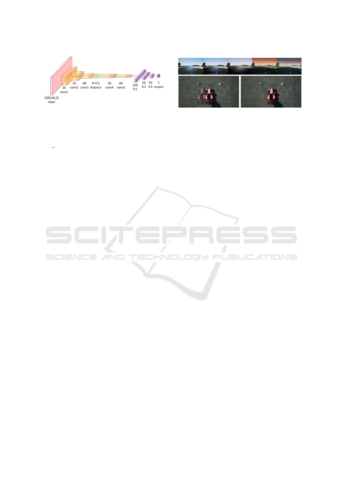
Figure 3: Illustration of our modified PilotNet. We added a
dropout layer (in green) in the middle of the convolutional
block, ReLU as activation functions after each hidden layer
and a Sigmoid activation function following the last layer.
ˆy ∈ [0, 1] as direct steering angle, instead of comput-
ing
1
ˆr
where ˆr is the circuit radius leading to the pre-
dicted steering. Also, we added ReLU activation fol-
lowing the hidden layers and a Dropout (Srivastava
et al., 2014) layer with a parameter p = 0.5. A lin-
ear normalization of the image is expected to be per-
formed by the users of the network prior to inference.
A scheme of the final network is shown in figure 3.
3.3 Augmentation and Data
Enhancements
Only a part of the recorded image is relevant in mak-
ing the decision of the appropriate steering angle.
Therefore, as shown in figure 1, we crop a region
of 200x66 pixels from the image that is fed into the
network. To promote generalization, we used meth-
ods of data distortion and adjustments on sampled im-
ages. The difference in light exposure between real-
world camera images to simulation recorded images
invoked a need for manual change of brightness level.
To address this, we duplicated the images in the pre-
processing phase in variations of up to 40% of the
original brightness. We also used various settings of
weather conditions when recording the data. These
settings include cloud opacity and prevalence, light
intensity and sun temperature. In addition, we used
several post-process distortion methods on some of
the sampled images. These included horizontal line
contribution, horizontal distortion and lens flare re-
flection.
We propose a novel method we call Shifted driv-
ing. Based on the idea of clipping an image and
post-processing the steering angle (Koppula, 2017),
we shift the camera’s position along the width of the
track and post-process the steering angle accordingly,
as illustrated in figure 4. Avoiding clipping an im-
age and instead maintaining the entire region of in-
terest, allows us to shift the camera’s position more
drastically. Our shifting distance in meters from the
center, d ∈ [−1.75, 1.75], is normally distributed with
zero mean. Using this method improved our ability
Figure 4: Illustration of our augmentation methods. Sam-
ples from CycleLight, a daylight cycle animation, demon-
strating the effect of the time of the day on the environment
(top). Shifted driving from a top view, illustrating the posi-
tion of the car after shifting the camera one meter to the left
(bottom).
to face difficult situations that the car sometimes got
into while self-driving and get back to the center of
the track. It had made a great contribution to the abil-
ity of our model to maintain reliable driving, as will
be discussed in sub-section 4.1. We also propose Cy-
cleLight, a novel method for introducing variation in
recorded driving data in a simulated environment. Cy-
cleLight, as illustrated in figure 4, is an animation of a
day-light cycle in a changeable, potentially very short
period of time, i.e., by turning this feature on during
recording session, we could collect images from dif-
ferent hours of the day in just a few minutes, instead
of manually recording a whole day in different condi-
tions. The usage of this feature caused the model to
become very robust to changes in shadowing condi-
tions, daytime vs nighttime, ad signs, tire walls etc.
3.4 Database and Recording Strategies
From different drivers, we chose three accurate and
well-trained drivers to record driving sessions. The
overall recording time for these drivers was approxi-
mately 220 minutes. We built several virtual tracks.
Almost half of the recorded data was taken from driv-
ing sessions on tracks which were mostly straight.
For the other recordings, we used curvy tracks in
which the number of left turns and the number of right
turns were balanced. Since our competition regula-
tions determine the distance between cones at each
side of the track to be between 300 and 500 cen-
timeters, we simulated different distances between
cones during our training procedure. Recordings were
done by purposely using two driving styles, norma-
tive and swerved. Normative driving is the sensi-
ble way of keeping close to the center line of the
road, while swerved driving means to constantly turn
sharply from one edge of the road to the other. With-
out swerved driving style, our recordings were safe
and steady, keeping close to the center of the road, not
able to learn extreme situations. This method served
Explorations and Lessons Learned in Building an Autonomous Formula SAE Car from Simulations
417
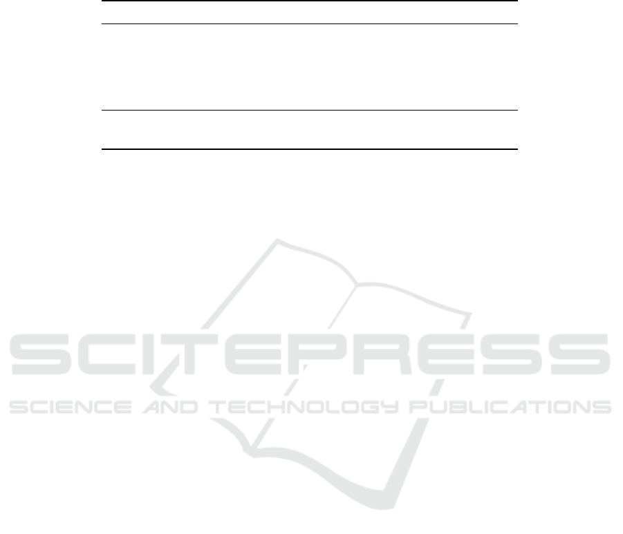
Table 1: Distribution for usage of the various techniques. Our augmentations contain methods to synthesize a given image,
e.g., adding distortions and reflections, along with our unique methods to vary the recording position and animate a day-light
cycle. Each percentage is related only to the mentioned technique, so overlaps between techniques are possible. The last
technique shows that we used an almost equal amount of data from mostly straight tracks and from tracks containing many
turns.
Type Method Percentage of usage
Augmentations
Horizontal line additions 10.0%
Horizontal distortion 11.4%
Light reflection 9.9%
CycleLight 77.2%
Shifted driving 22.2%
Recording techniques
Swerved driving 7.5%
Curvy/straight-line 46.1% / 53.9%
the purpose of adding data samples of the car driving
to the edge of the road and returning to the center.
3.5 Real World Setup
The need to react quickly in racing competitions
raises the importance of performing decision making
in high frequencies. Such tasks, and especially tasks
involving deep learning strategies, require an effi-
cient computer that can manage parallel computations
while operating under low-power constraints. While
our entire training procedure was based on Keras, an
API that is not supported in some computer archi-
tectures, running our trained model on such comput-
ers required a transition of the model to TensorFlow
framework. To increase the number of frames per sec-
ond, we optimized our pre-processing phase. The op-
timization included cropping the relevant ROI from a
given image prior to processing and replacing previ-
ous computations. The improvements in performance
of such transition are described in section 4.3 and are
shown in table 3. Our final program operates in 45
frames per second on average.
As for our camera, we used a single colored cam-
era with a specific lens as the input device. The lens
has a FOV (field of view) of 60
◦
, like the simulated
one, but it is vulnerable to changes in lighting expo-
sure. Instead of manually adjusting the exposure, we
used a software-based auto-exposure method. Then,
we shipped our steering decisions using a serial port
to the next stage, a micro-controller, that instructed
the car’s steering mechanism in combination with
other dynamic constraints.
4 EXPERIMENTS
For testing our models, we used tracks with specifica-
tions that are dictated by the competition regulations.
The simulation test-track featured driving at noon-
time on mostly straight roads. The track included del-
icate turns, small hills, and shades. The car throttle
value was determined by a function linear in the steer-
ing angle. One lap took 11 minutes of driving, with a
maximum speed of approximately 25 km/h. The met-
ric used for benchmarking was the time passed from
the moment the car started driving until it drove out of
the track, as seen in table 2 and discussed in section
4.1. The experiments composed of various changes
in the initial PilotNet architecture, as demonstrated in
figure 3, and shown in table 2. In the real-world, the
time of day for testing was mostly noon. We held two
different experiments, one is a completely straight-
line road and the second is a wave-like curved track.
During our benchmarking procedures, we tried
different modifications to the network. Table 2 shows
the main points of change along with our training pro-
cedure from the perspective of data distribution and
architecture. In contrary to what would seem to be
the normative way of using a test set, we based our
estimation of how good a model is by letting it drive
through specific unseen tracks. This was done since
there is more than one correct way to drive, thus hav-
ing a test set would not necessarily generate proper
feedback. Addition of a Dropout layer produced an
improvement in model performance, as mentioned in
table 2. Also, a Sigmoid activation was added to the
end of the network as an output normalizer.
After experiments with and without the car state,
i.e., brakes, throttle, speed and previous steering as
additional input, we observed over-fitting in the for-
mer case. e.g., after adding the swerved style data,
the model was driving out of the center of the track
more frequently and the performance worsened. The
experiments described in table 2 show improvement
after removing the car state. We observed that it was
better to discard these as inputs, despite their signif-
icance to the problem description. After the addition
SIMULTECH 2019 - 9th International Conference on Simulation and Modeling Methodologies, Technologies and Applications
418
of shifted driving, the final model performed excep-
tionally well on previously unseen tracks, as shown in
table 2. Some of these tracks included objects beside
the road. In all of these experiments, the car main-
tained an average speed of roughly 25 km per hour.
4.1 Simulation Experiments
Table 2: Comparison of our milestones throughout the ex-
periments. We evaluate the model by measuring the time
from the moment the car starts driving until it drives out of
the track. When using a test set that is composed from a
human recording, we observed that there is weak correla-
tion between the evaluation loss and the driving behaviour.
For example, adding the shifted driving method substan-
tially enhanced the model’s efficiency, an insight which we
couldn’t infer using a natural test set.
Modifications Duration
Original PilotNet 20 seconds
Dropout, Leaky ReLU 3 minutes
Addition of swerved data 5 minutes
Removal of car state 6 minutes
Shifted driving 3 hours
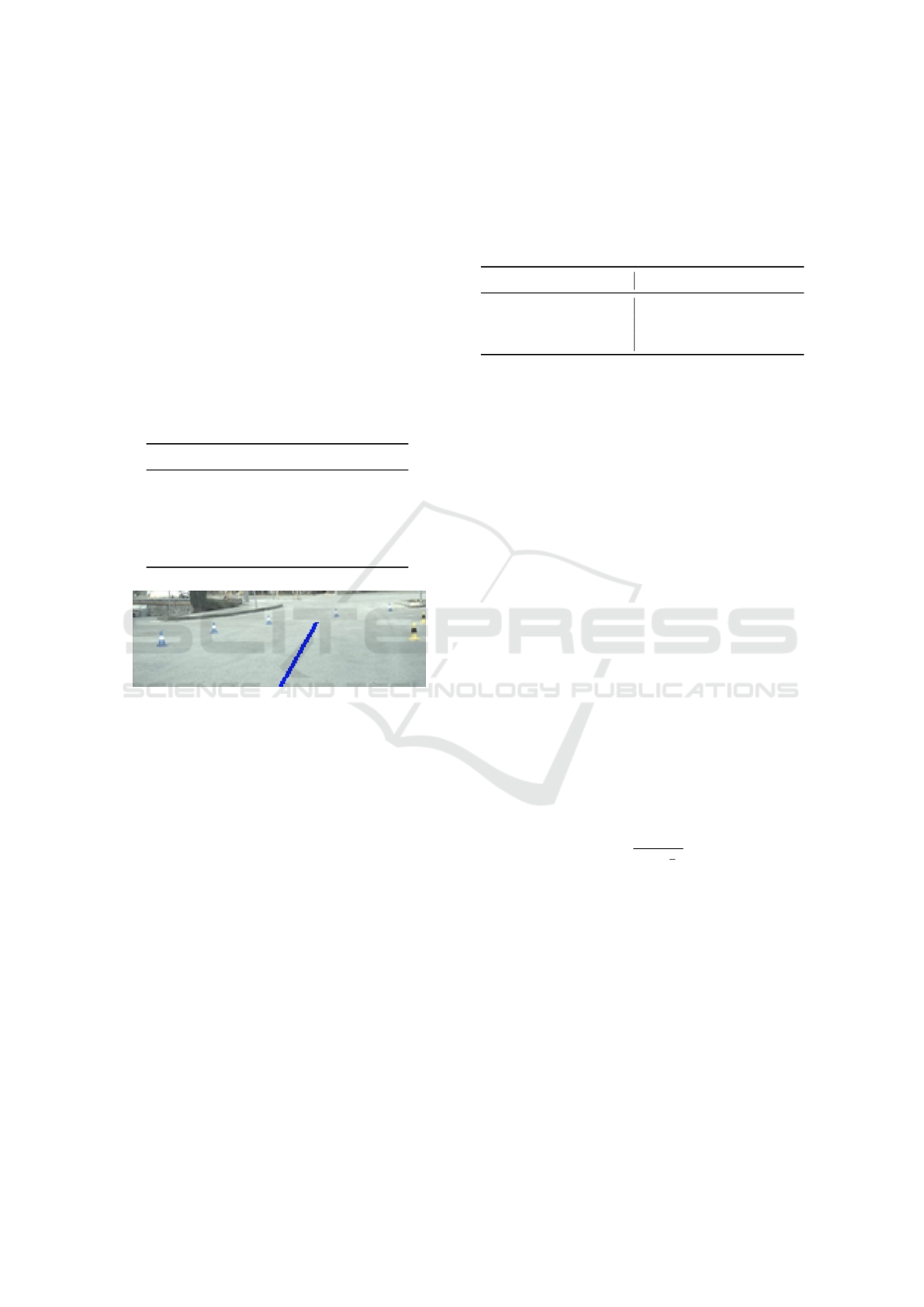
Figure 5: A sample taken from a recorded video in a parking
lot. The predicted steering angle is marked with a blue line
on the image. At this stage, the trained model from the
simulation is tested on the video, without any conversions.
4.2 Transition from Simulation to Real
World
To ensure the precision of the model in the real world,
we tested it offline on given videos of driving on a
closed-off road track. Due to the lack of labels in our
videos, we conducted these experiments using the fol-
lowing procedure: we marked the predicted steering
angles on the videos using a drawn line, as shown
in figure 5. We were assisted by experts from the
dynamic team of the car who tested the videos and
helped us to realize if the predicted steering angles
had the expected directions.
As mentioned before, we needed to convert our
model to TensorFlow framework and optimize re-
sponse time. To check the validity of the transi-
tion, we tested both Keras and TensorFlow models
on given videos. We compared the inference results
of both models, assuming they should produce the
Table 3: Execution of one hundred samples in both comput-
ers, running on three different code implementations. On
the left column is a desktop computer containing Nvidia
Geforce GTX1080, while on the right is a Nvidia Jet-
son TX2. The results are presented in average execution
time per iteration, in seconds. Due to lack of support, we
couldn’t evaluate Keras inference on TX2.
x86 TX2
Keras inference 0.0026 sec -
TensorFlow inference 0.0351 sec 0.4174 sec
Optimized inference 0.0025 sec 0.0176 sec
same outputs. Also, we checked the inference time
in both cases. We took one hundred samples and let
both computers execute inference on them. As shown
in table 3, we assured that our optimized code can
execute sufficient inference frequencies on our desig-
nated computer.
4.3 Real World Experiments
For the sake of simplicity, we began by using a
“clean” environment, i.e., one that included only our
Jetson TX2 computer, a camera, a micro-controller
and traffic cones in a lab, despite many differences
from an outdoor road scene. This helped us in avoid-
ing the interruptions of mechanical issues within the
car. We set the experiments by placing traffic cones
in the lab’s open space in different positions, to create
various indoor track segments.
We investigated the effects of changing the cam-
era’s parameters and realized that FOV, aperture di-
ameter, shutter speed and color scheme influenced the
most. To adjust the attributes of the camera to align
with the simulated one, we calculated f , the focal
length of the lens which depends on x, the FOV of
the simulated camera, and on d, the diameter of the
sensor:
f =
d
2tan(
x
2
)
(1)
Where in our case d equals to 11.345 mm and x equals
to 60
◦
. To prove the necessity in using the same pa-
rameters of the camera in real-world like the simu-
lated one, we conducted an experiment in a lab using
two different cameras. One that had a FOV of 60
◦
,
like the simulated one and the other with a FOV of
64
◦
. We placed traffic cones in two rows in front of
the cameras and installed both cameras in the same
position, in several rotations. We were expecting to
find a meaningful pattern with respect to the direc-
tion values. The results showed us a less spiked be-
havior in the slope of the graph for the camera with
the same FOV as the simulated one, which means a
smooth tendency in the difference between predicted
Explorations and Lessons Learned in Building an Autonomous Formula SAE Car from Simulations
419
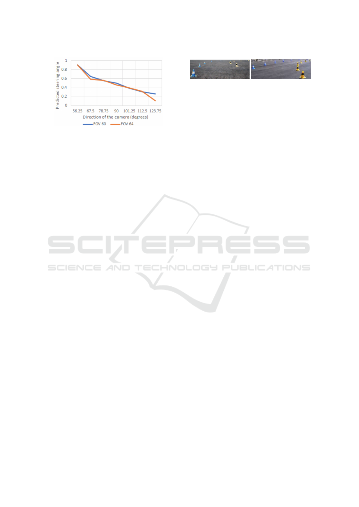
Figure 6: Predicted steering angle as a function of place-
ment direction of the cameras. The graph shows the differ-
ence between two chosen cameras.
steering angles. This is shown in figure 6.
To distinguish between the execution of the pro-
gram to the mechanical work of the controller, we
tested the connection to the controller without using
the actual car. This experiment was performed using
an Arduino module as a micro-controller receiving
the output from our Jetson TX2, and presenting the
predicted value using a LED light bulb. Our next step
was the outdoor scene. At first, the experiments were
held statically in a closed-off road scene. We placed
a work-station in different positions, consisting of the
Jetson TX2 and the camera, which were placed on a
track marked by traffic cones. The camera’s height
was adjusted to its original height on the actual car.
This was the first time we encountered sensitive ex-
posure, this led us to correct the exposure using pro-
grammatic auto-exposure solutions.
The last experiments took place on a parking lot
and finally on an obstacle-free road segment, using
the actual car. The speed was increased progressively.
To cope with the operations of mechanical systems,
such as clutch and throttle control, we were forced to
test the program’s performance with slow speeds. The
best way to do so was without ignition while turning
on the steering system alone. One of the main prob-
lems was a delay in steering execution. The dynamic
model of the steering mechanism was under construc-
tion until our experiments phase, hence the simulated
model did not consider the mechanical delay times
accurately. Sending a steering value from the model
to the controller took negligible time while mechan-
ically changing the direction of the wheels took two
times longer than expected. Thus, executing the steer-
ing angle instruction was slow, the car consistently
drove out of track and the car’s attempts to get back
on track were unsuccessful. After a trial and error pro-
cedure, we managed to identify the optimal driving
speed, which was 15-20 km/h, limited by mechanical
constrains.
Also, we encountered dazzling when driving in a
specific time of the day, in different directions. Such
Figure 7: Comparison between sampled images taken from
our simulated camera (left) and our real world camera
(right).
phenomena resulted in unwanted anomalies during
inference, which often led us to abort the driving un-
willingly. One way of dealing with such a problem is
to use multiple cameras or additional camera filters.
Also, the usage of distance estimators, e.g., Lidar or
depth cameras, can help overcome such distortions in
real world images. The driving results in real-world
were highly successful with the model trained on data
gathered from simulation only. The car drove better
than expected and was able to finish track segments
of 100-200 meters long.
5 DISCUSSION
A prominent aspect of what makes our training pro-
cedure interesting is the fact that no real-world data
was used, this greatly simplified the data gathering
process. Augmentation and recording techniques that
were used to compensate for the lack of real-world
data, proved to be crucial for the successful transition
of the model to the actual car. Also noteworthy is the
fact that no depth related sensor was used in any part
of our work, moreover, we managed to implement a
well-performing algorithm using only a single cam-
era as our input, an uncommon practice in the self-
driving field. Finally, we have also shown that such
algorithms can run under low-power constraints in a
sufficiently high enough throughput.
At a broader sense than previously discussed, the
concepts we used during our training procedure could
be deployed when attempting a variety of different
tasks. One could think of utilizing CycleLight to
varying lighting conditions when training off-road
vehicles to maneuver between obstacles, or rethink-
ing the idea of shifted driving to spread out on a
two-dimensional space when training trajectory plan-
ning for air crafts. On such cases, we believe that
simulation-based training would greatly simplify the
process.
ACKNOWLEDGEMENTS
The research was sopported by the Intelligent Sys-
tems Lab (ISL) and the Center for Graphics and Ge-
ometric Computing (CGGC), CS faculty, Technion.
SIMULTECH 2019 - 9th International Conference on Simulation and Modeling Methodologies, Technologies and Applications
420

The Formula SAE car was supplied by the Technion
Formula Student Team.
REFERENCES
Bast, H., Delling, D., Goldberg, A. V., M
¨
uller-Hannemann,
M., Pajor, T., Sanders, P., Wagner, D., and Werneck,
R. F. (2016). Route planning in transportation net-
works.
Bojarski, M., Del Testa, D., Dworakowski, D., Firner,
B., Flepp, B., Goyal, P., Jackel, L. D., Monfort,
M., Muller, U., Zhang, J., et al. (2016). End to
end learning for self-driving cars. arXiv preprint
arXiv:1604.07316.
Brubaker, M. A., Geiger, A., and Urtasun, R. (2016). Map-
based probabilistic visual self-localization. IEEE
Trans. Pattern Anal. Mach. Intell., 38(4):652–665.
Chebotar, Y., Handa, A., Makoviychuk, V., Macklin, M., Is-
sac, J., Ratliff, N. D., and Fox, D. (2018). Closing the
sim-to-real loop: Adapting simulation randomization
with real world experience. CoRR, abs/1810.05687.
Chen, L., Papandreou, G., Kokkinos, I., Murphy, K., and
Yuille, A. L. (2017). Deeplab: Semantic image seg-
mentation with deep convolutional nets, atrous convo-
lution, and fully connected crfs. CoRR, 2017 IEEE
Transactions on Pattern Analysis and Machine Intel-
ligence, abs/1606.00915.
Codevilla, F., Miiller, M., L
´
opez, A., Koltun, V., and Doso-
vitskiy, A. (2018). End-to-end driving via conditional
imitation learning. In 2018 IEEE International Con-
ference on Robotics and Automation (ICRA), pages 1–
9. IEEE.
Glassner, Y., Gispan, L., Ayash, A., and Shohet, T. F.
(2019). Closing the gap towards end-to-end au-
tonomous vehicle system. CoRR, abs/1901.00114.
James, S., Wohlhart, P., Kalakrishnan, M., Kalash-
nikov, D., Irpan, A., Ibarz, J., Levine, S., Had-
sell, R., and Bousmalis, K. (2018). Sim-to-real
via sim-to-sim: Data-efficient robotic grasping via
randomized-to-canonical adaptation networks. CoRR,
abs/1812.07252.
Kiran, B. R., Rold
˜
ao, L., Irastorza, B., Verastegui, R., S
¨
uss,
S., Yogamani, S., Talpaert, V., Lepoutre, A., and Tre-
hard, G. (2018). Real-time dynamic object detection
for autonomous driving using prior 3d-maps. CoRR,
ECCV 2018.
Koppula, S. (2017). Learning a cnn-based end-to-end
controller for a formula sae racecar. arXiv preprint
arXiv:1708.02215.
Levinson, J. and Thrun, S. (2010). Robust vehicle localiza-
tion in urban environments using probabilistic maps.
2010 IEEE International Conference on Robotics and
Automation, pages 4372–4378.
Li, P., Chen, X., and Shen, S. (2019). Stereo R-CNN based
3d object detection for autonomous driving. CoRR,
abs/1902.09738.
Mehta, A., Subramanian, A., and Subramanian, A.
(2018). Learning end-to-end autonomous driv-
ing using guided auxiliary supervision. CoRR,
abs/1808.10393.
Peng, X. B., Andrychowicz, M., Zaremba, W., and Abbeel,
P. (2017). Sim-to-real transfer of robotic control with
dynamics randomization. CoRR, abs/1710.06537.
Redmon, J., Divvala, S. K., Girshick, R. B., and Farhadi, A.
(2015). You only look once: Unified, real-time object
detection. CoRR, abs/1506.02640.
Shah, S., Dey, D., Lovett, C., and Kapoor, A. (2018). Air-
sim: High-fidelity visual and physical simulation for
autonomous vehicles. In Field and service robotics,
pages 621–635. Springer.
Srivastava, N., Hinton, G., Krizhevsky, A., Sutskever, I.,
and Salakhutdinov, R. (2014). Dropout: a simple way
to prevent neural networks from overfitting. The Jour-
nal of Machine Learning Research, 15(1):1929–1958.
Tan, J., Zhang, T., Coumans, E., Iscen, A., Bai, Y., Hafner,
D., Bohez, S., and Vanhoucke, V. (2018). Sim-to-
real: Learning agile locomotion for quadruped robots.
CoRR, abs/1804.10332.
Urmson, C., Anhalt, J., Bagnell, D., Baker, C., Bittner, R.,
Clark, M., Dolan, J., Duggins, D., Galatali, T., Geyer,
C., et al. (2008). Autonomous driving in urban envi-
ronments: Boss and the urban challenge. Journal of
Field Robotics, 25(8):425–466.
Valls, M. I., Hendrikx, H. F., Reijgwart, V. J., Meier, F. V.,
Sa, I., Dub
´
e, R., Gawel, A., B
¨
urki, M., and Siegwart,
R. (2018). Design of an autonomous racecar: Percep-
tion, state estimation and system integration. In 2018
IEEE International Conference on Robotics and Au-
tomation (ICRA), pages 2048–2055. IEEE.
Xu, Y., John, V., Mita, S., Tehrani, H., Ishimaru, K., and
Nishino, S. (2017). 3d point cloud map based vehicle
localization using stereo camera. 2017 IEEE Intelli-
gent Vehicles Symposium (IV).
You, Y., Pan, X., Wang, Z., and Lu, C. (2017). Virtual to
real reinforcement learning for autonomous driving.
BNVC.
Explorations and Lessons Learned in Building an Autonomous Formula SAE Car from Simulations
421
