
A Multiobjective Artificial Bee Colony Algorithm based on
Decomposition
Guang Peng, Zhihao Shang and Katinka Wolter
Department of Mathematics and Computer Science, Free University of Berlin, Takustr. 9, Berlin, Germany
Keywords:
Multiobjective Optimization, Evolutionary Computation, Decomposition, Artificial Bee Colony, Adaptive
Normalization.
Abstract:
This paper presents a multiobjective artificial bee colony (ABC) algorithm using the decomposition approach
for improving the performance of MOEA/D (multiobjective evolutionary algorithm based on decomposi-
tion). Using a novel reproduction operator inspired by ABC, we propose MOEA/D-ABC, a new version
of MOEA/D. Then, a modified Tchebycheff approach is adopted to achieve higher diversity of the solutions.
Further, an adaptive normalization operator can be incorporated into MOEA/D-ABC to solve the differently
scaled problems. The proposed MOEA/D-ABC is compared to several state-of-the-art algorithms on two
well-known test suites. The experimental results show that MOEA/D-ABC exhibits better convergence and
diversity than other MOEA/D algorithms on most instances.
1 INTRODUCTION
In many real-life applications, a decision maker needs
to handle different conflicting objectives. Problems
with more than one conflicting objectives are called
multiobjective optimization problems (MOPs). Mul-
tiobjective evolutionary algorithms (MOEAs) have
been developed for solving MOPs (Deb and Kalyan-
moy, 2001). MOEA based on decomposition
(MOEA/D) (Zhang and Li, 2007) is a novel MOEA
framework, which decomposes a MOP into a series of
scalar optimization problems. Recently, the MOEA/D
framework has achieved great success and received
much attention (Trivedi et al., 2017). We focus on
the following three aspects of existing research stud-
ies about MOEA/D.
Research on other nature inspired meta-heuristics
combined with MOEA/D is increasing. Based on
the MOEA/D framework, Li and Landa-Silva (Li and
Landa-Silva, 2011) incorporated simulated annealing
to propose a MOEA for solving multiobjective knap-
sack problems. Moubayed et al. (Al Moubayed
et al., 2014) adopted particle swarm optimization to
develop decomposition-based multiobjective particle
swarm optimizers. Ke et al. (Ke et al., 2013) pro-
posed a MOEA using decomposition and ant colony
optimization.
Decomposition approaches have also been widely
studied. In the original MOEA/D (Zhang and Li,
2007) there are three decomposition methods includ-
ing the weighted sum approach, the weighted Tcheby-
cheff approach and the penalty-based boundary inter-
section (PBI) approach. To deal with the poor di-
versity control problem of the original Tchebycheff
approach, Qi et al. (Qi et al., 2014) put forward
a transformed Tchebycheff approach, which substi-
tutes the weight vector by its respective “normaliza-
tion inverse”. The transformed Tchebycheff approach
can obtain better uniformly distributed solutions com-
pared with the original Tchebycheff approach. Hi-
royuki et al. (Sato, 2015) used a nadir point to pro-
pose an inverted PBI approach for solving multiob-
jective maximization problems. Zhang et al. (Zhang
et al., 2018) developed a modified PBI approach for
MOPs with complex Pareto fronts.
Since the original MOEA/D is sensitive to the
scales of objectives, some normalization operators
need to be incorporated into the MOEA/D framework.
In MOEA/D (Zhang and Li, 2007), a simple normal-
ization method is used to replace the original objec-
tives. NSGA-III (Deb and Jain, 2014) designs an
achievement scalarizing function to get the extreme
points to constitute a hyperplane, and uses the inter-
cepts on each axis to normalize the objectives. Unlike
NSGA-III, I-DBEA (Asafuddoula et al., 2014) adopts
a corner-sort-ranking procedure to calculate the ex-
treme points to build the hyperplane, and also uses
the intercepts to normalize the objectives. Compared
188
Peng, G., Shang, Z. and Wolter, K.
A Multiobjective Artificial Bee Colony Algorithm based on Decomposition.
DOI: 10.5220/0008167801880195
In Proceedings of the 11th International Joint Conference on Computational Intelligence (IJCCI 2019), pages 188-195
ISBN: 978-989-758-384-1
Copyright
c
2019 by SCITEPRESS – Science and Technology Publications, Lda. All rights reserved

with the usual normalization method in MOEA/D,
both procedures based on hyperplanes (Deb and Jain,
2014)(Asafuddoula et al., 2014) are more computa-
tionally expensive for solving the linear system of
equations. Moreover, these two procedures are not
used for biobjectives.
Following the above ideas, three objectives are
followed in this paper: first, we want to develop other
nature inspired meta-heuristics so as to adopt an arti-
ficial bee colony algorithm as the reproduction opera-
tor to improve the performance of MOEA/D. Second,
we substitute the original Tchebycheff approach with
a modified Tchebycheff approach for improved diver-
sity. Then, in terms of differently scaled problems,
an adaptive normalization mechanism is incorporated
into the proposed algorithm. Finally, we propose a
multiobjective artificial bee colony algorithm based
decomposition for the different MOPs.
The rest of this paper is organized as follows.
The technical background is presented in Section 2
and the details of the proposed algorithm are pre-
sented in Section 3. The performance of the pro-
posed MOEA/D-ABC on two well-known test suites
is presented and compared with other state-of-the-art
MOEAs in Section 4. The final section summarizes
the contributions and points to future research.
2 BACKGROUND
In this section, some basic concepts behind MOP are
provided. Then, we briefly introduce the most widely
used decomposition methods and the original artifi-
cial bee colony algorithm, respectively.
2.1 Multiobjective Optimization
A MOP can be defined as follows (Reyes-Sierra et al.,
2006):
min F(x) = ( f
1
(x), f
2
(x),··· , f
m
(x))
T
(1)
subject to x ∈ Ω ⊆ R
n
where Ω is the decision space and x = (x
1
,x
2
,··· ,x
n
)
is an n-dimensional decision vector; F : Ω → Θ ⊆ R
m
denotes an m-dimensional objective vector and Θ is
the objective space.
Definition 1 (Pareto Dominance). A decision vector
x
0
=
x
0
1
,x
0
2
,··· ,x
0
n
is said to dominate another deci-
sion vector x
1
=
x
1
1
,x
1
2
,··· ,x
1
n
, denoted by x
0
≺ x
1
,
if
f
i
x
0
≤ f
i
x
1
, ∀i ∈
{
1,2,··· ,m
}
f
j
x
0
< f
j
x
1
, ∃ j ∈
{
1,2,··· ,m
}
(2)
Definition 2 (Pareto Optimal Solution). A solution
vector x
0
=
x
0
1
,x
0
2
,··· ,x
0
n
is called a Pareto optimal
solution, if ¬∃x
1
: x
1
≺ x
0
.
Definition 3 (Pareto Optimal Solution Set). The
set of Pareto optimal solutions is defined as
PS =
x
0
¬∃x
1
≺ x
0
.
Definition 4 (Pareto Front). The Pareto op-
timal solution set in the objective space
is called Pareto front, denoted PF =
{
F (x) = ( f
1
(x), f
2
(x),··· , f
m
(x))
|
x ∈ PS
}
.
2.2 Decomposition Approach
MOEA/D is an efficient algorithm framework ap-
proaching the Pareto front. The weighted sum ap-
proach, the Tchebycheff approach and the PBI ap-
proach are three widely used decomposition meth-
ods in the framework. It has been proven that the
weighted sum approach does not work well with non-
convex Pareto fronts.
In the Tchebycheff approach a scalar optimization
problem can be stated as follows:
min
x∈Ω
g
te
(x
|
λ,z
∗
)=min
x∈Ω
max
1≤i≤m
{
λ
i
|
f
i
(x) − z
i
∗
|}
(3)
where λ = (λ
1
,λ
2
,··· ,λ
m
)
T
is a weight vec-
tor and
∑
m
i=1
λ
i
= 1,λ
i
≥ 0,i = 1,2,··· ,m. z
∗
=
(z
∗
1
,z
∗
2
,··· ,z
∗
m
)
T
is the reference point. Because it is
often time-consuming to compute the exact z
∗
i
, it is
estimated by the minimum objective value f
i
(i.e.,
z
∗
i
=min
{
f
i
(x)
|
x ∈ Ω
}
,i = 1,2,··· ,m).
A scalar optimization problem of the PBI ap-
proach is defined as follows:
min
x∈Ω
g
pbi
(x
|
λ,z
∗
) = min
x∈Ω
(d
1
+ θd
2
) (4)
where
d
1
=
k
( f (x)−z
∗
)
T
λ
k
k
λ
k
d
2
=
f (x) −
z
∗
+ d
1
λ
k
λ
k
(5)
Here θ is a user-predefined penalty parameter. d
1
denotes the distance of the projection of vector
( f (x) − z
∗
) along the weight vector. d
2
denotes the
perpendicular distance from f (x) to λ.
2.3 The Artificial Bee Colony Algorithm
The Artificial bee colony (ABC) algorithm is a pop-
ulation based algorithm, which is motivated by the
intelligent foraging behavior of a honey bee swarm
(Karaboga, 2005). The honey bee colony swarm con-
tains three types of bees: employed bees, onlooker
bees, and scout bees.
A Multiobjective Artificial Bee Colony Algorithm based on Decomposition
189

In the ABC algorithm, the number of employ-
ees and onlookers is equal to the number of food
sources. The ABC algorithm first generates a ran-
domly distributed initial population of N solutions.
Then, the employed bees search the new solutions
within the neighborhood in their memory. Let X
i
=
{
x
i,1
,x
i,2
,··· ,x
i,n
}
represent the i-th solution in the
swarm, where n is the dimension. Each employed bee
X
i
generates a new position V
i
using the following for-
mula:
V
i,k
= X
i,k
+ Φ
i,k
×
X
i,k
− X
j,k
(6)
where X
j
is a randomly selected solution (i 6= j),k is
a random dimension index from the set
{
1,2,··· ,n
}
,
and Φ
i,k
is a random number within the range [−1,1].
After generating a new candidate solution V
i
, a greedy
selection between V
i
and X
i
is used. Comparing the
fitness value between V
i
and X
i
, the better one is
adopted to update the population. Once the search-
ing phase of the employed bees is completed, the em-
ployed bees share the food source information with
the onlooker bees through waggle dances. An on-
looker bee chooses a food source with a probability
based on a roulette wheel selection mechanism. The
probability P
i
for the maximization problem is defined
as follows:
P
i
=
f it
i
∑
N
j
f it
j
(7)
where f it
i
is the fitness value of the i-th solution. The
better solution often has higher probability to be cho-
sen to reproduce the new solution using Eq. 6. If a
position X
i
cannot be improved through a predefined
number of cycles, then it is replaced by the new so-
lution X
new
i
discovered by the scout bee using the fol-
lowing equation:
X
new
i,k
= lb
i
+ rand(0,1) × (ub
i
− lb
i
) (8)
where rand(0,1) is a random number in [0,1]. The
upper and lower boundaries of the i-th dimension are
lb
i
and ub
i
, respectively.
3 THE PROPOSED ALGORITHM
In this section we will present the details of the new
algorithm proposed in this paper.
3.1 Overview
The general framework of the proposed MOEA/D-
ABC is given in Algorithm 17. First, a
set of uniformly distributed weight vectors Λ =
λ
1
,λ
2
,··· ,λ
N
is generated (Zhang and Li, 2007).
Then, a population of N solutions P =
{
x
1
,x
2
,··· ,x
N
}
is initialized randomly, after that the reference point
z
∗
= (z
∗
1
,z
∗
2
,··· ,z
∗
m
)
T
is initialized. According to the
generated weight vectors, the neighborhood range T
of subproblem i as B (i) =
{
i
1
,··· ,i
T
}
can be obtained
by computing the Euclidean distance between all the
weight vectors and finding the T closest weight vec-
tors. Steps 7-17 are iterated until the termination cri-
terion is met. At each iteration, for the solution x
i
, the
mating solutions x
k
and x
l
are chosen from the neigh-
borhood B(i). In MOEA/D-ABC, we use the ABC
operator and polynomial mutation operator to repro-
duce the offspring y, which will be introduced in de-
tail in Section 3.3. Then the new offspring is used
to update the reference point and neighboring solu-
tions. In addition, we use the modified Tchebycheff
approach to determine the search direction for updat-
ing the neighboring solutions.
Algorithm 1: Framework of MOEA/D-ABC.
1 Generate a set of weight vector
Λ ←
λ
1
,λ
2
,··· ,λ
N
;
2 Initialize the population P ←
{
x
1
,x
2
,··· ,x
N
}
;
3 Initialize the reference point
z
∗
← (z
∗
1
,z
∗
2
,··· ,z
∗
m
)
T
;
4 for i = 1 : N do
5 B(i) ←
{
i
1
,i
2
,··· ,i
T
}
, where
λ
i
1
,λ
i
2
,··· ,λ
i
T
are T closest weight
vectors to λ
i
;
6 end
7 while the termination criterion is not satisfied
do
8 for i = 1 : N do
9 E ← B (i) ;
10 Select an index k ∈ E based on
roulette wheel selection ;
11 Randomly select an index l ∈ E and
l 6= k ;
12 ¯y ← ABCOperator (x
k
,x
l
);
13 y ← PolynomialMutationOperator ( ¯y);
14 UpdateIdealPoint(y,z
∗
);
15 UpdateNeighborhood(y,z
∗
,Λ,B(i));
16 end
17 end
3.2 Modified Tchebycheff Approach
In MOEA/D-ABC, we adopt the modified Tcheby-
cheff approach, which is defined as follows:
min
x∈Ω
g
mte
(x
|
λ,z
∗
)=min
x∈Ω
max
1≤i≤m
1
λ
i
|
f
i
(x) − z
i
∗
|
(9)
ECTA 2019 - 11th International Conference on Evolutionary Computation Theory and Applications
190

where λ = (λ
1
,λ
2
,··· ,λ
m
)
T
is a weight vec-
tor and
∑
m
i=1
λ
i
= 1,λ
i
≥ 0,i = 1,2,··· ,m. z
∗
=
(z
∗
1
,z
∗
2
,··· ,z
∗
m
)
T
is the reference point. It is worth not-
ing that the modified Tchebycheff approach has two
advantages (Yuan et al., 2015) over the original one
in MOEA/D (Zhang and Li, 2007). First, the modi-
fied form can produce more uniformly distributed so-
lutions with a set of uniformly spread weight vectors.
Second, each weight vector corresponds to a unique
solution on the Pareto front (PF). The proof can be
found in Theorem 1.
Theorem 1. Assume the straight line passing through
reference point z
∗
with the direction vector λ =
(λ
1
,λ
2
,...,λ
m
)
T
has a intersection with the PF, then
the intersection point is the optimal solution to Γ(x)
(i.e., Γ(x) = max
1≤i≤m
n
1
λ
i
|
f
i
(x) − z
i
∗
|
o
).
Proof. Let F (x) be the intersection point with the PF,
then we can have the following equality
f
1
(x) − z
∗
1
λ
1
=
f
2
(x) − z
∗
2
λ
2
= ··· =
f
m
(x) − z
∗
m
λ
m
= C
(10)
where C is a constant. Suppose F (x) that is not the
optimal solution to Γ(x), then ∃F (y) satisfies Γ(y) <
Γ(x). According to Eq. 10, Γ(x) = C. Then ∀k ∈
{
1,2,··· ,m
}
, we have
f
k
(y) − z
∗
k
λ
k
≤ Γ(y) < C =
f
k
(x) − z
∗
k
λ
k
(11)
Hence, f
k
(y) < f
k
(x). This is in contradiction
with the condition that F (x) is the intersection point
on the PF and the supposition is invalid.
3.3 The ABC Operator
Inspired by the ABC algorithm, we adopt the ABC
operator to reproduce the offspring. For each solu-
tion x
i
, one mating solution x
k
is chosen based on
the roulette wheel selection mechanism and another
x
l
(l 6= k) is randomly selected from the neighborhood
B(i). To get the mating solution x
k
, assuming there is
a solution x
i
and its associated weight vector λ
i
. First,
the fitness value of the solution x
i
can be calculated
using the following equation:
Γ(x
i
) = max
1≤ j≤m
(
1
λ
i
j
f
j
(x
i
) − z
j
∗
)
(12)
In this way we can obtain T fitness values Γ (B (i))
of the neighboring solutions with the same weight
vector λ
i
. Then the fitness value of the solution x
i
can be converted in the following way:
Γ
∗
(x
i
) = exp
−Γ(x
i
)
∑
Γ(B(i))
T
!
(13)
According to the converted T fitness values the
mating solution x
k
can be determined using the
roulette wheel selection mechanism. For each solu-
tion x
i
, the new solution ¯y is computed as follows:
¯y = x
k
+ Φ
i
× (x
k
− x
l
) (14)
where Φ
i
is a n-dimensional random vector within the
range [−1,1]. After using the ABC operator to obtain
the new solution ¯y, we apply a polynomial mutation
operator (Deb and Kalyanmoy, 2001) on ¯y to produce
a new offspring y.
3.4 Adaptive Normalization
For disparately scaled objectives the original
MOEA/D sometimes cannot provide satisfying
results. The normalization operators are by default
incorporated into the MOEA/D framework. In
recent research there are three typical normalization
approaches proposed in MOEA/D (Zhang and Li,
2007), NSGA-III (Deb and Jain, 2014), and I-DBEA
(Asafuddoula et al., 2014). The normalization
procedures in NSGA-III and I-DBEA are similar to
some extent, as both aim to find the extreme points
to constitute a hyperplane. However, these two
algorithms are more computationally expensive for
solving the linear system of equations and sometimes
result in abnormal normalization results (Yuan et al.,
2014). Therefore, in this paper we select a simple
and efficient way to normalize the objectives.
For a solution x
i
the objective value
f
j
(x
i
) ( j = 1,2,··· ,m) can be replaced with the
normalized objective value
¯
f
j
(x
i
) as follows:
¯
f
j
(x
i
) =
f
j
(x
i
) − z
∗
j
z
max
j
− z
∗
j
(15)
where z
max
j
is the maximum value of objective f
j
in
the current population.
3.5 Computational Complexity
For MOEA/D-ABC, the major computational costs
are the iteration process in the Algorithm 17. Step
9-13 mainly need O (mT ) operations to calculate
the modified Tchebycheff values for choosing the
mating solutions based on the roulette wheel selec-
tion mechanism. Step 14 performs O (m) compar-
isons to update the reference point. Step 15 re-
quires O (mT ) computations to update the neighbor-
hood. Thus, the overall computational complexity of
MOEA/D-ABC is O(mNT ) in one generation. Con-
sidering the adaptive normalization operator incorpo-
rated into the MOEA/D-ABC for solving the scaled
optimization problems, the computational complexity
A Multiobjective Artificial Bee Colony Algorithm based on Decomposition
191

of MOEA/D-ABC will be O
mN
2
in one generation
since T is smaller than N.
4 EXPERIMENTAL STUDIES
In this section we compare the performance of
the proposed algorithm with other state-of-the-art
MOEAs for solving different MOPs.
4.1 Experiment Settings
The proposed MOEA/D-ABC is implemented in the
PlatEMO framework (Tian et al., 2017). For better
comparison the other algorithms are also chosen from
the PlatEMO. Two well-known ZDT (Zitzler et al.,
2000) and DTLZ (Deb et al., 2001) test suites are used
as test instances.
In order to evaluate the performance of the pro-
posed algorithm, we have chosen the inverse genera-
tional distance (IGD) (Veldhuizen and Lamont, 1998)
as a performance metric which can reflect both con-
vergence and diversity. Since the exact Pareto front of
the test problems is known we can easily locate some
uniformly targeted points in the optimal surface. Let
P
∗
be a set of these uniformly targeted points. Let A
be a set of final non-dominated solutions in the objec-
tive space, which can be obtained for each algorithm.
The IGD metric is computed as follows:
IGD(A,P
∗
) =
1
|
P
∗
|
v
u
u
t
|
P
∗
|
∑
i=1
˜
d
2
i
(16)
where
˜
d
i
is the Euclidean distance between the i-th
member of the set P
∗
and its nearest member in the
set A. As for the IGD metric the smaller value means
the obtained solutions have better quality. For each
test instance 30 independent runs are performed and
mean and standard deviation of the IGD values are
recorded. For all algorithms we use the solutions from
the final generation to compute the performance met-
rics.
In the experiment the performance of MOEA/D-
ABC is compared with NSGA-II (Deb et al., 2002),
MOEA/D (Zhang and Li, 2007) and MOEA/D-DE
(Li and Zhang, 2009). The original MOEA/D
study proposes two procedures MOEA/D-TCH us-
ing the Tchebycheff and MOEA/D-PBI using the
PBI approach. Table 1 presents some parameters for
crossover and mutation operators used in MOEA/D-
ABC, NSGA-II, MOEA/D-TCH and MOEA/D-DE.
The other additional parameters are set according
to suggestions given by their original papers. The
Table 1: Parameters for crossover and mutation.
Parameters MOEA/D-ABC NSGA-II MOEA/D-TCH MOEA/D-DE
SBX probability (p
c
) - 1 1 -
Polynomial mutation probability (p
m
) 1/n 1/n 1/n 1/n
Distribution index for crossover (η
c
) - 20 20 -
Distribution index for mutation (η
m
) 20 20 20 20
DE operator control parameter (CR) - - - 1
DE operator control parameter (F) - - - 0.5
neighborhood size T is set to be 20 and the penalty pa-
rameter θ is set to 5 for MOEA/D-PBI. In MOEA/D-
DE the probability δ of choosing the parent solution
form the whole population is set to 0.9 and the max-
imum number of replaced solutions n
r
is set to 2. As
analyzed above MOEA/D-ABC has the obvious ad-
vantage of having less parameters.
4.2 Normalized Test Problems
Initially we use the ZDT problems and the DTLZ
problems (DTLZ1, DTLZ2, DTLZ3, DTLZ4) to test
the performance of the respectively used algorithms.
The number of variables D is set according to the
original papers. Since the test problems have similar
range of values for each objective they are called “nor-
malized test problems”. For all 2-objective (m = 2)
ZDT test problems the population size N in NSGA-II
and other variants of MOEA/D is set to be 100 and the
number of function evaluations (FEs) is set as 30000.
For all 3-objective (m = 3) DTLZ test problems N is
set to 200 and FEs is set to 100000.
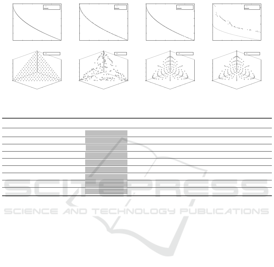
Fig. 1 shows the obtained fronts with the median
value of IGD performance metric of all algorithms
for ZDT4 and DTLZ1. From Fig. 1 we can observe
that the proposed algorithm MOEA/D-ABC can de-
termine the Pareto optimal solutions with better con-
vergence and diversity. Compared with the other three
algorithms MOEA/D-DE has the worst convergence
for the ZDT4 problem with its many local optima.
NSGA-II can determine the random non-dominated
solutions in the Pareto front. Both MOEA/D-TCH
and MOEA/D-DE use the Tchebycheff approach as
decomposition method to obtain the similar Pareto
front. MOEA/D-ABC performs much better than
MOEA/D-TCH and MOEA/D-DE with regard to the
diversity which illustrates that the modified Tcheby-
cheff approach improves the diversity of MOEA/D
compared with the original Tchebycheff approach.
Table 2 shows that MOEA/D-ABC outperforms the
other three algorithms with respect to the IGD perfor-
mance metric.
4.3 Scaled Test Problems
To investigate the proposed algorithm’s performance
in the case of disparately scaled objectives we choose
the modified ZDT1 and ZDT2 as two two-objective
test instances and DTLZ1 and DTLZ2 as the two
ECTA 2019 - 11th International Conference on Evolutionary Computation Theory and Applications
192
0 0.2 0.4 0.6 0.8 1
f
1
0
0.2
0.4
0.6
0.8
1
f
2
ZDT4
MOEA/D-ABC
PF
0 0.2 0.4 0.6 0.8 1
f
1
0
0.2
0.4
0.6
0.8
1
f
2
ZDT4
NSGA-II
PF
0 0.2 0.4 0.6 0.8 1
f
1
0
0.2
0.4
0.6
0.8
1
f
2
ZDT4
MOEA/D-TCH
PF
0 0.2 0.4 0.6 0.8 1
f
1
0
0.5
1
1.5
2
f
2
ZDT4
MOEA/D-DE
PF
0
00
0.1
0.2
f
3
DTLZ1
0.3
0.2
0.2
f
1
f
2
0.4
0.5
0.4
0.4
MOEA/D-ABC
0
0 0
0.1
0.2
f
3
DTLZ1
0.3
0.2
0.2
f
1
f
2
0.4
0.5
0.4
0.4
NSGA-II
00
0.1
0.10.1
0.2
DTLZ1
f
3
0.3
0.20.2
f
1
f
2
0.4
0.30.3
0.5
0.40.4
MOEA/D-TCH
0
0 0
0.1
0.2
DTLZ1
f
3
0.3
0.2
0.2
f
2
f
1
0.4
0.5
0.4
0.4
MOEA/D-DE
Figure 1: Obtained solutions by MOEA/D-ABC, NSGA-II, MOEA/D-TCH, and MOEA/D-DE for ZDT4 and DTLZ1.
Table 2: IGD values for MOEA/D-ABC, NSGA-II, MOEA/D-TCH, and MOEA/D-DE on ZDT and DTLZ.
Problem N m D FEs MOEA/D-ABC NSGA-II MOEA/D-TCH MOEA/D-DE
ZDT1
100 2 30 30000 4.0371e-3 (6.09e-5) 4.6043e-3 (1.84e-4) 5.8106e-3 (5.88e-3) 1.1626e-2 (5.42e-3)
ZDT2
100 2 30 30000 3.8379e-3 (2.29e-5) 4.7864e-3 (1.99e-4) 5.3845e-3 (4.66e-3) 9.4609e-3 (3.62e-3)
ZDT3
100 2 30 30000 1.0928e-2 (3.85e-2) 4.1278e-2 (5.03e-2) 1.9680e-2 (2.06e-2) 2.5511e-2 (1.52e-2)
ZDT4
100 2 10 30000 4.5511e-3 (9.93e-4) 5.4563e-3 (9.52e-4) 7.3588e-3 (4.00e-3) 1.8529e-1 (1.62e-1)
ZDT6
100 2 10 30000 3.1078e-3 (1.07e-5) 3.7673e-3 (1.14e-4) 3.1968e-3 (4.79e-5) 3.1125e-3 (1.63e-5)
DTLZ1
200 3 7 100000 1.4208e-2 (6.95e-4) 1.9097e-2 (9.01e-4) 1.9937e-2 (2.02e-5) 1.9716e-2 (5.19e-5)
DTLZ2
200 3 12 100000 3.7745e-2 (3.05e-4) 4.8807e-2 (1.49e-3) 4.9259e-2 (7.96e-5) 4.8923e-2 (2.25e-4)
DTLZ3
200 3 12 100000 4.3475e-2 (2.96e-3) 4.8337e-2 (1.22e-3) 4.8881e-2 (2.52e-4) 1.3899e-1 (4.83e-1)
DTLZ4
200 3 12 100000 4.1621e-2 (1.35e-3) 4.8543e-2 (1.33e-3) 2.7569e-1 (2.73e-1) 7.3774e-2 (6.23e-2)
three-objective test instances. The modified objective
f
i
is multiplied with a factor 10
i−1
. For example, ob-
jectives f
1
, f
2
and f
3
for the three-objective scaled
DTLZ1 problem are multiplied with 10
0
, 10
1
and 10
2
,
respectively.
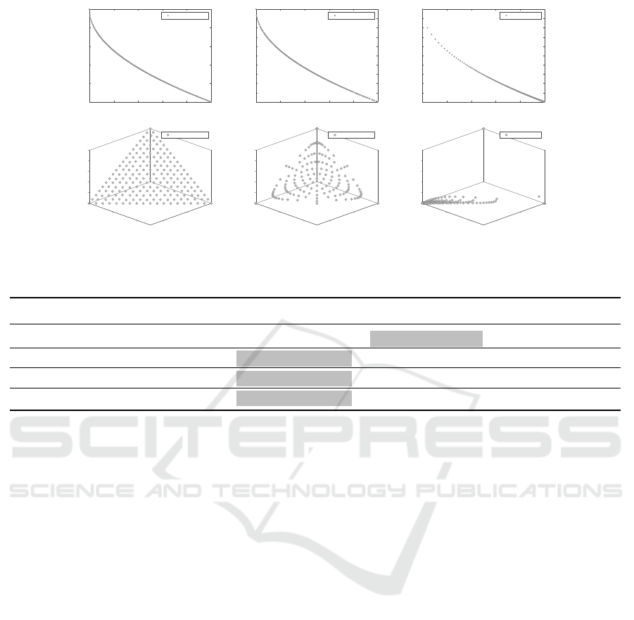
To handle the differently scaled test problems, we
incorporate the adaptive normalization operator pre-
sented in Section 3.4 into the proposed MOEA/D-
ABC. The original MOEA/D-TCH with and without
normalization procedure is also used to compare the
performance. For clarity, we denote the MOEA/D-
ABC using the normalization procedure as MOEA/D-
ABC-N, MOEA/D-TCH with normalization proce-
dure as MOEA/D-TCH-N, respectively. Fig. 2 shows
the distribution of obtained solutions for MOEA/D-
ABC-N, MOEA/D-TCH-N and MOEA/D-TCH on
scaled ZDT1 and DTLZ1. It is clear that the normal-
ization operator can greatly improve the performance
for handling the scaled problems. Both MOEA/D-
ABC-N and MOEA/D-TCH-N can obtain better dis-
tributed solutions than MOEA/D-TCH with regard to
two-objective test instances. MOEA/D-TCH is not
able to handle the differently scaled DTLZ1 with-
out normalization. It is interesting to observe that
MOEA/D-ABC-N is superior to MOEA/D-TCH-N
with respect to diversity for solving three-objective
test instances. The IGD performance metric val-
ues of concerning algorithms are shown in Table 3
which also verifies the efficiency and reliability of
MOEA/D-ABC with normalization for solving dis-
parately scaled objective problems.
4.4 MOEA/D-ABC vs MOEA/D-PBI
In the original MOEA/D study (Zhang and Li,
2007), MOEA/D-PBI can obtain much better distri-
bution of solutions than NSGA-II and MOEA/D-TCH
on DTLZ1 and DTLZ2 instances when setting the
penalty parameter as 5. According to the experiments
on normalized test problems, MOEA/D-ABC can
also get good results on three-objective instances. To
further compare the performance of MOEA/D-ABC
and MOEA/D-PBI, we choose DTLZ5 and DTLZ6
as the test instances.
Fig. 3 shows the obtained Pareto fronts with
MOEA/D-ABC and MOEA/D-PBI on DTLZ5. It is
clear that MOEA/D-PBI is unable to find the con-
vergent front with the penalty factor 5. However,
MOEA/D-ABC can determine the front approach-
ing the true Pareto front. Table 4 shows the IGD
metric of the obtained solutions with MOEA/D-ABC
and MOEA/D-PBI for DTLZ5 and DTLZ6 instances.
A Multiobjective Artificial Bee Colony Algorithm based on Decomposition
193
0 0.2 0.4 0.6 0.8 1
f
1
0
2
4
6
8
10
f
2
ZDT1
MOEA/D-ABC-N
0 0.2 0.4 0.6 0.8 1
f
1
1
2
3
4
5
6
7
8
9
10
f
2
ZDT1
MOEA/D-TCH-N
0 0.2 0.4 0.6 0.8 1
f
1
1
2
3
4
5
6
7
8
9
10
f
2
ZDT1
MOEA/D-TCH
0
0 0
10
20
f
3
DTLZ1
30
0.2
2
f
1
f
2
40
50
0.4
4
MOEA/D-ABC-N
0
0 0
10
20
f
3
DTLZ1
30
2 0.2
f
2
f
1
40
50
4
0.4
MOEA/D-TCH-N
0
0 0
10
20
DTLZ1
f
3
30
2 0.2
f
2
f
1
40
4 0.4
MOEA/D-TCH
Figure 2: Obtained solutions by MOEA/D-ABC-N, MOEA/D-TCH-N, and MOEA/D-TCH for scaled ZDT1 and DTLZ1.
Table 3: IGD values for MOEA/D-ABC-N, MOEA/D-TCH-N, and MOEA/D-TCH on scaled ZDT1-2 and DTLZ1-2.
Problem N m D FEs MOEA/D-ABC-N MOEA/D-TCH-N MOEA/D-TCH
ZDT1
200 2 30 100000 1.1069e-2 (3.68e-5) 1.1043e-2 (7.72e-6) 5.0087e-2(6.85e-5)
ZDT2
200 2 30 100000 1.1358e-2 (1.14e-5) 6.8675e-1 (1.42e+0) 4.0293e-2(8.80e-6)
DTLZ1
200 3 7 100000 1.2620e-1 (2.06e-2) 5.2850e-1 (5.72e-3) 9.1805e+0(8.39e-3)
DTLZ2
200 3 12 100000 3.1699e-1 (2.07e-2) 1.0600e+0 (2.27e-3) 1.5530e+1(9.49e-3)
Based on the above result analysis we see that the
use of a penalty parameter cannot always obtain good
results. MOEA/D-PBI requires an appropriate set-
ting of the penalty parameter for different problems.
MOEA/D-ABC is a more stable and efficient algo-
rithm to solve different optimization problems.
5 CONCLUSIONS AND FUTURE
WORK
In this paper we have developed a multiobjective
artificial bee colony algorithm based on decompo-
sition for solving multiobjective optimization prob-
lems. The proposed MOEA/D-ABC approach adopts
a novel ABC operator as new reproduction operator
and a modified Tchebycheff approach as new decom-
position method, respectively. The above two opera-
tors are used to improve the convergence and diver-
sity of the algorithm. Furthermore, the adaptive nor-
malization operator is incorporated into the proposed
MOEA/D-ABC for handling differently scaled prob-
lems.
In the experiment two well-known test suites and
some modified scaled test instances are applied to
test the performance of proposed MOEA/D-ABC and
compare them with other state-of-the-art MOEAs.
The test problems involve fronts that have convex,
concave, disjointed, non-uniformly distributed, dif-
ferently scaled, and many local fronts where an op-
timization algorithm can get stuck in. The pro-
posed MOEA/D-ABC can obtain a well-converging
and well-diversified set of solutions repeatedly for all
problems, which shows its obvious advantage over
other state-of-the-art MOEAs. Moreover, there is
another advantage of MOEA/D-ABC which is that
it does not require any additional parameters with
respect to the reproduction operator compared with
other versions of MOEA/Ds.
In the future we will study the performance
of the proposed MOEA/D-ABC for solving many-
objective problems with more than three objectives. It
would also be interesting to study how the proposed
MOEA/D-ABC performs in practice.
REFERENCES
Al Moubayed, N., Petrovski, A., and McCall, J. (2014).
D2mopso: Mopso based on decomposition and dom-
inance with archiving using crowding distance in ob-
jective and solution spaces. Evolutionary computa-
tion, 22(1):47–77.
Asafuddoula, M., Ray, T., and Sarker, R. (2014).
A decomposition-based evolutionary algorithm for
many objective optimization. IEEE Transactions on
Evolutionary Computation, 19(3):445–460.
ECTA 2019 - 11th International Conference on Evolutionary Computation Theory and Applications
194
0
0.2
0.4
0.20.2
DTLZ5
f
3
0.6
f
1
f
2
0.8
0.40.4
1
0.60.6
MOEA/D-ABC
0
0.5
0.5
0.5
1
1
DTLZ5
f
3
f
1
f
2
1
1.5
1.5
2
2
2.5
2.5
MOEA/D-PBI
Figure 3: Obtained solutions by MOEA/D-ABC, and MOEA/D-PBI for DTLZ5.
Table 4: IGD values for MOEA/D-ABC, and MOEA/D-PBI on DTLZ5 and DTLZ6.
Problem N m D FEs MOEA/D-ABC MOEA/D-PBI
DTLZ5
200 3 12 100000 1.1250e-2 (2.06e-5) 2.2605e-2 (1.95e-5)
DTLZ6
200 3 12 100000 1.1319e-2 (7.43e-6) 2.2632e-2 (4.78e-6)
Deb, K. and Jain, H. (2014). An evolutionary many-
objective optimization algorithm using reference-
point-based nondominated sorting approach, part i:
solving problems with box constraints. IEEE Transac-
tions on Evolutionary Computation, 18(4):577–601.
Deb, K. and Kalyanmoy, D. (2001). Multi-Objective Opti-
mization Using Evolutionary Algorithms. John Wiley
& Sons, Inc., New York, NY, USA.
Deb, K., Pratap, A., Agarwal, S., and Meyarivan, T. (2002).
A fast and elitist multiobjective genetic algorithm:
Nsga-ii. IEEE Transactions on Evolutionary Compu-
tation, 6(2):182–197.
Deb, K., Thiele, L., Laumanns, M., and Zitzler, E.
(2001). Scalable test problems for evolutionary multi-
objective optimization. Technical report, Computer
Engineering and Networks Laboratory (TIK), Swiss
Federal Institute of Technology (ETH.
Karaboga, D. (2005). An idea based on honey bee swarm
for numerical optimization.
Ke, L., Zhang, Q., and Battiti, R. (2013). Moea/d-aco: A
multiobjective evolutionary algorithm using decom-
position and antcolony. IEEE transactions on cyber-
netics, 43(6):1845–1859.
Li, H. and Landa-Silva, D. (2011). An adaptive evolution-
ary multi-objective approach based on simulated an-
nealing. Evolutionary Computation, 19(4):561–595.
Li, H. and Zhang, Q. (2009). Multiobjective optimization
problems with complicated pareto sets, moea/d and
nsga-ii. IEEE Transactions on Evolutionary Compu-
tation, 13(2):284–302.
Qi, Y., Ma, X., Liu, F., Jiao, L., Sun, J., and Wu, J. (2014).
Moea/d with adaptive weight adjustment. Evolution-
ary computation, 22(2):231–264.
Reyes-Sierra, M., Coello, C. C., et al. (2006). Multi-
objective particle swarm optimizers: A survey of the
state-of-the-art. International journal of computa-
tional intelligence research, 2(3):287–308.
Sato, H. (2015). Analysis of inverted pbi and compari-
son with other scalarizing functions in decomposition
based moeas. Journal of Heuristics, 21(6):819–849.
Tian, Y., Cheng, R., Zhang, X., and Jin, Y. (2017). Platemo:
A matlab platform for evolutionary multi-objective
optimization [educational forum]. IEEE Computa-
tional Intelligence Magazine, 12:73–87.
Trivedi, A., Srinivasan, D., Sanyal, K., and Ghosh, A.
(2017). A survey of multiobjective evolutionary al-
gorithms based on decomposition. IEEE Transactions
on Evolutionary Computation, 21(3):440–462.
Veldhuizen, D. A. V. and Lamont, G. B. (1998). Multiob-
jective evolutionary algorithm research: A history and
analysis.
Yuan, Y., Xu, H., and Wang, B. (2014). An improved nsga-
iii procedure for evolutionary many-objective opti-
mization. In Proceedings of the 2014 Annual Con-
ference on Genetic and Evolutionary Computation,
GECCO ’14, pages 661–668, New York, NY, USA.
ACM.
Yuan, Y., Xu, H., Wang, B., Zhang, B., and Yao,
X. (2015). Balancing convergence and diversity
in decomposition-based many-objective optimizers.
IEEE Transactions on Evolutionary Computation,
20(2):180–198.
Zhang, Q. and Li, H. (2007). Moea/d: A multiob-
jective evolutionary algorithm based on decomposi-
tion. IEEE Transactions on evolutionary computation,
11(6):712–731.
Zhang, Q., Zhu, W., Liao, B., Chen, X., and Cai, L. (2018).
A modified pbi approach for multi-objective optimiza-
tion with complex pareto fronts. Swarm and Evolu-
tionary Computation, 40:216–237.
Zitzler, E., Deb, K., and Thiele, L. (2000). Comparison
of multiobjective evolutionary algorithms: Empirical
results. Evol. Comput., 8(2):173–195.
A Multiobjective Artificial Bee Colony Algorithm based on Decomposition
195
