Multivariate Time Series Forecasting with Deep Learning Proceedings in

Energy Consumption

edra Mellouli

1 a

, Mahdjouba Akerma

, Minh Hoang

, Denis Leducq

and Anthony Delahaye

LIASD EA4383, IUT de Montreuil, Universit

e Paris 8, Vincennes Saint-Denis, France

Irstea, UR GPAN, Anthony, France

Keywords:

Demand Response, Deep Learning, Time Series Forecasting.

Abstract:

We propose to study the dynamic behavior of indoor temperature and energy consumption in a cold room

during demand response periods. Demand response is a method that consists of smoothing demand over time,

seeking to reduce or even stop consumption during periods of high demand in order to shift it to periods

of lower demand. Such a system can therefore be tackled as the study of a time-series, where each behav-

ioral parameter is a time-varying parameter. Different network topologies are considered, as well as existing

approaches for solving multi-step ahead prediction problems. The predictive performance of short-term pre-

dictors is also examined with regard to prediction horizon. The performance of the predictors are evaluated

using measured data from real scale buildings, showing promising results for the development of accurate

prediction tools.

1 INTRODUCTION

In France as elsewhere in the world, the balance be-

tween electricity production and consumption is a ne-

cessity that must be maintained and for which elec-

tricity suppliers are required to index electricity pro-

duction to the demand of grid users. To do this,

suppliers must regularly deploy more production re-

sources with fast response times. In addition, the Eu-

ropean Union has set itself the target of increasing the

share of renewable energy in energy consumption to

27% by 2030, from 17% in 2016. However, these new

means of production, whose productivity may vary

according to time of day, season or climate, require

a rethinking of the use of the global electricity grid

to allow more ﬂexibility. Due to this high complex-

ity and when the main objective is the ﬁnal result ob-

tained at the output of the system independently of in-

ternal operation, it may be interesting to examine the

use of Black Box models, the purpose is to predict

the output parameters according to the inputs. The

study of the dynamic behavior of such a system can

therefore be approached as the study of a time series,

where each behavioral parameter is a time-varying pa-

rameter. A time series is a sequence of real-valued

signals that are measured at successive time inter-

https://orcid.org/0000-0001-8858-9902

vals. Long short-term memory (LSTM)(Hochreiter

and Schmidhuber, 1997), a class of recurrent neural

networks (RNNs)(andY. Bengio and Hinton, 2015),

is particularly designed for sequential data. For time

series prediction task LSTM has particularly shown

promising results. Four deep neural network architec-

tures derived from the LSTM architecture were stud-

ied, adapted and compared. Their validation was car-

ried out using experimental data collected in a cold

room in order to evaluate their performance in pre-

dicting demand response. In this paper, we present

our methodology allows us to effectively answer the

following questions:1) Which deep learning models

are best suited to represent our speciﬁc data? 2) From

the selected models, we have sought to deﬁne and

characterize the most efﬁcient predictive models and

to highlight all the parameters that induce them. 3) In

addition to their relevance, we are looking to evaluate

the robustness of the selected models at the last iter-

ation against the data quality (noise), data temporal

window scaling and large scaling data. The paper is

structered as following. In the next section we present

the related work, then we detail our approach. Finally

we describe the datasets used to compare four deep

leraning architectures and we discuss their results.

384

Mellouli, N., Akerma, M., Hoang, M., Leducq, D. and Delahaye, A.

Multivariate Time Series Forecasting with Deep Learning Proceedings in Energy Consumption.

DOI: 10.5220/0008168203840391

In Proceedings of the 11th International Joint Conference on Knowledge Discovery, Knowledge Engineering and Knowledge Management (IC3K 2019), pages 384-391

ISBN: 978-989-758-382-7

2 RELATED WORK

2.1 Time Series Models in Electrical

Demand Response Prediction

Time series is deﬁned as a sequence of discrete time

data. It consists of indexed data points, measured typ-

ically at successive times, spaced at (often uniform)

time intervals. Time series analysis comprises the dif-

ferent methods for analyzing such time series in order

to understand the theory behind the data points, i.e. its

characteristics and the statistical meaning (Nataraja

et al., 2012). A time series forecasting model pre-

dicts future values based on known past events (recent

observations). Conventional time series prediction

methods commonly use a moving average model that

can be autoregressive (ARMA)(Rojo-Alvarez et al.,

2004), integrated autoregressive (ARIMA) (Hamil-

ton, 1994) or vector autoregressive (VARMA)(Rios-

Moreno et al., 2007), in order to reduce data. Such

methods must process all available data in order to

extract the model parameters that best match the new

data. These methods are useless in the face of mas-

sive data and real-time series forecasting. To ad-

dress this problem, online time learning methods have

emerged to sequentially extract representations of un-

derlying models from time series data. Unlike tradi-

tional batch learning methods, online learning meth-

ods avoid unnecessary cost retraining when process-

ing new data. Due to their effectiveness and scalabil-

ity, online learning methods, including linear model-

based methods, ensemble learning and kernels, have

been successfully applied to time series forecasting.

Each time series forecasting model could have many

forms and could be applied to many applications.

For more detailes we can see (Amjady, 2001) (Aman

et al., 2015).

In our application context, (Hagan and Behr,

1987) have been reviewed time series based models

for load forecasting. Then in 2001 (Amjady, 2001)

has studied time series modeling for short to medium

term load forecasting. To predict energy consump-

tion some authors have used time series data. For

example, (J.W et al., 2006) have concentrated their

study on the comparison of the performance of the

methods for short-term electricity demand forecast-

ing using a time series. (Simmhan et al., 2013) have

focused their study on prediction of energy consump-

tion using incremental time series clustering, (Sheng

and Duc-Sonand, 2018) have also forecasted the en-

ergy consumption time series using machine learning

techniques. In (Aman et al., 2015) the work is fo-

cused on increasing the accuracy of prediction mod-

els for dynamic demand response, this prediction is

based on a very small data granularity (15 min inter-

vals). The focus on demand response has been on

large industrial and commercial consumers (Ziekow

et al., 2013) which are expected by their high con-

tribution and adopted for the smart meters (Simmhan

et al., 2013).

2.2 Nonlinear Models

Due to the very high complexity and need for accu-

racy that the use of linear modeling, which is very

time-consuming, can imply, the transition to another

more applied type of modeling can simplify the study.

Indeed, when the main objective is the ﬁnal result ob-

tained at the output of a system, regardless of internal

operation, it may be interesting to look at the use of

non-linear models, whose purpose is solely to predict

the output parameters from the inputs. This presents

in addition the advantage of being much more easily

generalizable, at least in the presence of data of sufﬁ-

cient good quality and by ﬁnding a model correspond-

ing to our problematic, without requiring a reshaping

of the problem and adaptation of the different param-

eters when studying a new system. In particular, Arti-

ﬁcial Neural Networks (ANN) could provide an alter-

native approach, as they are widely accepted as a very

promising technology offering a new way to solve

complex problems. ANNs ability in mapping com-

plex non-linear relationships, have succeeded in sev-

eral problems such as planning, control, analysis and

design. The literature has demonstrated their superior

capability over conventional methods, their main ad-

vantage being the high potential to model non-linear

processes, such as utility loads or energy consump-

tion in individual buildings . At present, although

studies (Hu et al., 2017)(Xue et al., 2014) have been

carried out within the wide framework of demand re-

sponse, no such method does appear to have been

applied to demand response in the ﬁeld of refriger-

ation. In consideration of the energy importance of

this ﬁeld which provides a panel of signiﬁcant op-

portunities, the use of a pertinent modelling approach

can demonstrate (or invalidate) the use of demand re-

sponse in cold rooms and cold stores, allowing (or

not) a signiﬁcant increase in the application of elec-

trical cut-off. An LSTM network, or ”Long Short

Term Memory”, is a model for retaining short-term

information (recent variations and current trends in

data) and long-term ones (periodicity, recurring or

non-recurring events). It is a matter of a deep learn-

ing model widely used for time series processing. It

is popular due to the ability of learning hidden long-

term sequential dependencies, which actually helps

in learning the underlying representations of time se-

Multivariate Time Series Forecasting with Deep Learning Proceedings in Energy Consumption

385

ries (Kuo and Huang, 2018).A convolutional LSTM

model was proposed based on the Fully Connected

LSTM model (Shi et al., 2015), particularly for its ap-

plication to predicting changes in spatial images. This

model has allowed them to obtain better results than

using a simple LSTM or Fully-Connected LSTM net-

work. The architecture of an LSTM network therefore

consists of a sequence of LSTM layers for both past

and future data, which are then processed together to

predict current data. To conclude, the modeling of a

refrigeration system being characterized by the non

linearity and the coupling of several parameters, clas-

sical physical models encounter difﬁculties in predict-

ing the dynamic behaviour of such systems, in par-

ticular during disturbances such as electrical cut-off

periods. Neural network methods, due to their abil-

ity to adjust and self learning, can therefore be very

promising in responding to this type of issues offering

a new way to solve complex problems. The LSTM

ability in mapping complex non-linear relationships,

have succeeded in several problems such as planning,

control, analysis and design of energy systems. The

literature has demonstrated their superior capability

over conventional methods, their main advantage be-

ing the high potential to model non-linear processes.

3 OUR APPROACH

3.1 Experimental Setup of Cold Room

A cold room or cold store ensures that the products

are kept in satisfactory conditions. This therefore re-

quires the use of a refrigeration system, which can

take the form of a regular supply of cold air, in order

to keep the air and products below a setpoint temper-

ature, generally below −18

◦

C. This phenomenon fol-

lows the refrigeration cycle, passing through its four

main stages, namely compression, condensation, ex-

pansion and evaporation. In order to avoid signiﬁcant

heat leakage, it is also necessary to reduce external in-

puts, through optimal thermal insulation and to min-

imize door openings as well as human or mechanical

activities 1. The products are stored in the form of

distributed pallets to reduce the phenomenon of natu-

ral warming while facilitating access to the products

during loading and unloading. The cold room used in

this study is about 2.4m long x 2.4m width x 2m high.

For wall insulation, a 10cm layer of polyurethane with

λ = 0.023W /m.K is used. A global heat transfer co-

efﬁcient Uc = 0.29W /m2K is obtained by measure-

ment. The room temperature is controlled using an

on/off strategy and is kept at −16.3

◦

C (within a lim-

ited range (set-point) between −15.5

◦

C and −19

◦

C).

The refrigerated unit consists of a single evaporator

with single speed fan. The measured coefﬁcient of

performance (COP) is 1.4 at -16

◦

C. The cold room

is installed inside an external cell equipped with an

air conditioning unit to simulate the meteorological

conditions (summer, spring. . . ). To limit the inﬁl-

tration load, the doorway is kept closed during mea-

surements. In order to measure the air and product

temperature, thermocouple sensors are used (Fig. 2).

These thermocouples are distributed as follows (cf.

Figure 1):

• 3 for cold blowing air (Ts) and 3 for return air (Tr)

• 14 for air temperature inside the cold room: 6 in

the middle of each wall, 1 near the door, 1 at one

wall surface (sample inside cold room), 6 at the

corners (2 other corners are not accessible by ther-

mocouples)

• 5 for air temperature in the external cell (Text) on

the surface of each wall

• Two wattmeters are used to measure the instanta-

neous electricity consumption of the refrigeration

system (compressor and auxiliary).

The main features of a cold room are of two cate-

gories. As a ﬁrst category, we ﬁnd ﬁxed features

which take into account building geometry (as build-

ing dimensions, wall thickness), building composition

(as material conductivity, density and overall heat ex-

change coefﬁcient), outdoor contributions (as outdoor

temperature, solar ﬂux, air renewal), cold production

(as setpoint temperature, blowing temperature, blow-

ing rate, operation of the refrigeration machine, cool-

ing capacity) and operations on building (as Loading,

product conductivity, product density, human pres-

ence, lighting, ventilation, defrosting, etc). The sec-

ond category includes mainly temporal features like

the demand response periods (T

erasure

) including both

the demand response phase itself (switching off the

cooling system) and the recovery phase of the cool-

ing system (restoring the set temperature); The de-

frost periods, (T

de f rost

) which occur several times a

day without any decision-making power on the time

of appearance. These periods correspond to a spe-

ciﬁc temperature increasing related to the defrost-

ing of the cold room fan; The compressor on/off

periods (compressor ), which occur very regularly

and on an ad hoc basis; The time elapsed since

the last demand response period (δT

erasure

), allow-

ing the model to better predict the behavior of the

cold room in the moments following the demand re-

sponse period, while its condition is not yet restored;

And the time elapsed since the last defrost (δT

de f rost

also allowing better prediction of the behaviour of

the cold room in the moments following defrosting,

KDIR 2019 - 11th International Conference on Knowledge Discovery and Information Retrieval

386

Figure 1: Example of a used cold room.

when the condition of the cold room is not yet stabi-

lized. According to the time parameters deﬁned be-

low we obtain a system with three modes behavior.

The ﬁrst mode (Fig.2(1))represents the steady state

where regular temperature variations according to set

points (high/low) are measured. The second mode

((Fig.2(2))is the critical state of the system refers to

electrical demand response. During this mode, the

temperature increases over a long period of time. This

period depends mainly on the demand response time

interval, typically varies between 30 minutes and 3

hours.The third mode ((Fig.2(3))is the defrost state in

which the temperature suddenly increases over a short

period of time.

3.2 Multivariate Electrical Demand

Response Data Time Series

In this section we deﬁne the list of time series data

we aim to predict. Indeed, we consider four data

classes. The ﬁrst class is dedicated to measure the

Indoor Temperature (T p

) using 5 sensors thus we

have ﬁve T p

time series. Sensors are located in

ﬁve strategic positions in the cold room. The second

class is the Recovery Temperature of the Air (T p

Air

)

in the cold room and we have three sensors to mea-

sure three T p

Air

time series. The third class is focused

to measure the Product Temperature (T p

Prod

) with 8

sensors and thus we have eight T p

Prod

) time series.

The last class is to measure the Outdoor Temperature

(T p

Out

using ﬁve sensors and we obtained ﬁve out-

door temperature time series. Compressor consump-

tion (Comp

nergy) which is a particular data time se-

ries correlated to the previous variable classes is also

considered. To solve the problems related to the si-

multaneous occurrence of defrosting and demand re-

sponse phenomena, i.e. the confusion of their mea-

surement periods, we have chosen to recover the de-

frosting and demand response programs directly by

observing the temperature variations that occur dur-

ing demand response period and defrosting. All time

series data are measured each ﬁve seconds.

3.3 LSTM Models to Forcasting

Electrical Demand Response

We note {t p

,t p

,...,t p

} a time series represent-

ing any parameter T p

in the output set where x ∈

{Air,In,Product}. Our predictive model learns use-

ful features from a set of time series parameters to

give a prediction

t p

that compares with t p

to update

itself, where t p

is the real value measured at time t

and

t p

is the time series data point forecasted at the

same time. As it is proved in the literature, Long Short

Term Memory (LSTM) is required for discovering

a dependence relationships between the time series

data by using specialized gating and memory mech-

anisms. For this purpose, we are aimed to compare

four LSTM models : LSTM, Convolutionnal LSTM,

Stacked LSTM, Bidirectional LSTM. As a ﬁrst model

we have used LSTM.

After a huge number of experiments following

several evaluations of the model, the parameters were

selected for this model:

• 1024 units are able to store enough information.

This choice was made balancing the learning time

and the quality of obtained prediction.

• A linear or SeLu activation function, giving us

better results than the other functions

• A cost function using the Root Mean Square Error

(RMSE),

The second model is stacked LSTM. The devel-

oped Stacked LSTM model is a modiﬁcation of the

LSTM network described above, with the addition of

several layers of LSTM.

For this purpose, and after experimental tests, the

selected model consists of a stack of three layers of

LSTM, namely: A ﬁrst layer of 1024 memory units,

allowing to store a large amount of information in the

short and long term; A second layer of 512 memory

units; A third layer, of 256 memory units;

Each layer of the network is separated from the

next layer by a dropout layer, allowing less overtrain-

ing and robust generalization results.

For the Bidirectional LSTM network, it consists

of a stack of two layers of LSTMs each with 512

memory units. This model thus created makes it pos-

sible to keep information related to both past and fu-

ture data.

The convolutional LSTM network was chosen

with the following parameters: 40 ﬁlters, correspond-

ing to the outputs of the convolutional part of the

model; A kernel size of 2x10, corresponding to the

dimensions of the convolution window; A normaliza-

tion layer, allowing to normalize the activations of the

convolutional LSTM layer.

Multivariate Time Series Forecasting with Deep Learning Proceedings in Energy Consumption

387

3.4 Performance Metric for Evaluation

In order to compare our different models and to se-

lect the appropriate model(s) for our study, different

criteria were implemented and computed. In the fol-

lowing, the reference values will be indicated by Y ,

the predicted values by

Y , the average of the refer-

ence values by

Y and the number of observations by

N. The Fit criterion is needed for measuring the prox-

imity between the reference values and the predicted

values. The closer its value is to 100%, the more

it indicates a correctly predicted variable. It there-

fore corresponds to a percentage and is deﬁned by:

Fit(Y ) = 100.(1 −

Y −Y|

|Y −

Y |

The Mean-Squared-Error (MSE), or mean square

error, is the arithmetic mean of the squares of the dif-

ferences between the forecasts and the actual obser-

vations. The objective of a good prediction is there-

fore to obtain the lowest possible mean square error.

The advantage of squaring is to highlight high errors,

and therefore to minimize low prediction errors. This

value is therefore deﬁned by: MSE(Y ) =

∑

i=1

(

−

)

. The root of this value, or Root-Mean-Squared-

Error (RMSE), is also often used, which is simply cal-

culated by: RMSE(Y ) =

MSE(Y ).

The Mean Absolute Error (MAE), or absolute

mean error, is the arithmetic mean of the differences

between forecasts and actual observations. Since

there is no squaring, this measure treats each dif-

ference with equal importance. The objective is

of course to minimize this value, and it is deﬁned

over prediction horizon [t + 1,t + H] by: MAE(Y ) =

∑

i=1

−Y

The coefﬁcient of variation (CV) is a little-known

measure that has been proposed by[Karatasou et al.,

2006][Amasyali et al., 2016] to evaluate the predic-

tion of models for building energy consumption. This

value is deﬁned as a percentage, by the formula :

CV (Y ) = 100.

RMSE(Y)

As this value is only used in the ﬁeld of energy

consumption, it will therefore only be evaluated on

consumption values, and not on temperatures (the lat-

ter may also be negative).

4 EXPERIMENTAL RESULTS

As mentioned above, we implemented the four LSTM

architectures described in the section 3.3. To evaluate

their performance in predicting demand response, a

set of use cases were developed based on experimen-

tal data collected in cold rooms. For the cold room,

we had access to large periods of measurement time

with acceptable accuracy where measurements were

made every ﬁve seconds. These measurements were

made in a cold room that was replicated in a con-

trolled environment to obtain data to form the models

and prove their predictive power. For these purposes,

we have proposed ﬁve use cases allowing us to an-

swer efﬁciently to the following questions :1) Which

deep learning models are more adapted to represent

our speciﬁc data? 2) Which model(s) is less sensitive

to the stochastic occurrence of electricity demand re-

sponse? 3) Which model(s) is more robust to the data

quality, i.e. signal noise (electrical demand response)

and horizon window? We assume that the reference

behaviour of a cold room is characterized by an ideal

”undisturbed” operation, with no phenomenon of de-

mand response or door opening and this over a long

period of time, in order to stabilize the internal tem-

perature. These data measurements are used only to

initialize the four architectures. Then we have estab-

lished ﬁve time series datasets to evaluate each LSTM

architecture. These datasets are described as follows.

We note by E

a dataset time series where i = 1..5

elaborated for each use case i:

• The use case 1 (train: 127975, test: 60000 )hy-

pothesis is to consider a set of measurements with

three electrical demand response periods, uni-

formly distributed over 3 days. Here we simulate

the stochastic disturbance of the system on con-

sidering a uniform distribution of the noise signal.

Hence δT

erasure

is randomly decreased and T

erasure

is ﬁxed ;

• The use case 2 (train: 223545, test: 149030) hy-

pothesis is to consider a set of measurements with

two electrical demand response periods per day,

uniformly distributed over 5 days. In this case we

increase the frequency of occurrence of the noise

in use case 1 and increase the total number of mea-

surements. Indeed, this case allows us to study the

bias of the frequency of noise occurrence as well

as the amount of data;

• The case 3 (train: 490985, test: 294590) hypoth-

esis is to consider a set of measurements over 5

days with one electrical demand response period

randomly occured per day and with a random pe-

riod. It means both δT

erasure

and T

erasure

are ran-

dom.

• The case 4 (train: 630920, test: 420610) hypoth-

esis is to consider the union of the three previ-

ous hypothesis. It corresponds to a generalized

model of the electrical demand response problem,

i.e. We have a large amount of data, more noise

and more randomness.

• The case 5 (train: 214080, test: 142700) hypoth-

KDIR 2019 - 11th International Conference on Knowledge Discovery and Information Retrieval

388

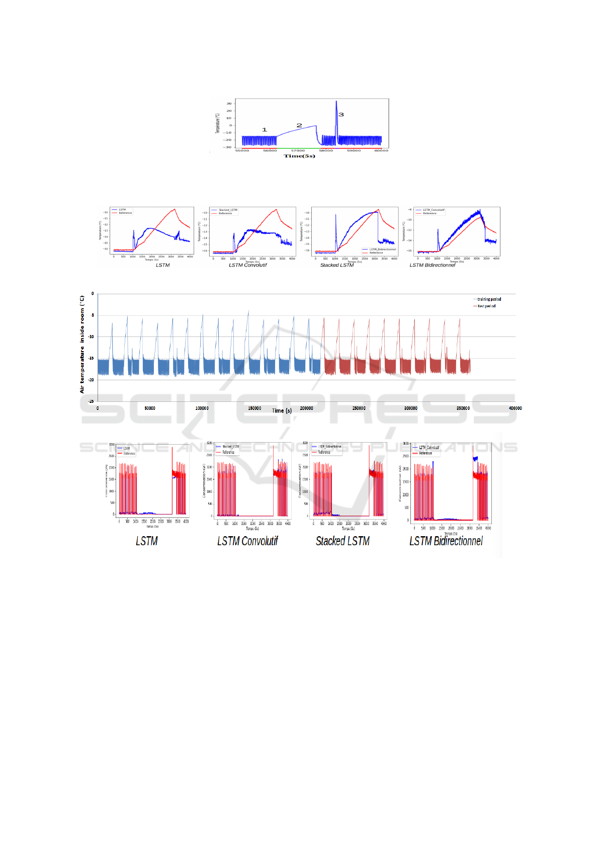
Figure 2: Three modes: (1)Steady state, regular temperature variations according to set points (high/low) ; (2)Electrical

demand response, temperature increases over a long period of time (30min-3h) ; (3)Defrosting, sudden temperature increase

for a very short time (5-10min).

Figure 3: LSTM models prediction of T p

product

in use case 1.

Figure 4: LSTM data time series prediction with E1 datasets.

Figure 5: LSTM models prediction of Compressor

Energy

in use case 1.

esis is to consider a ﬁxed δT

erasure

, a ﬁxed T

erasure

varing between 1 and 3 hours and we increase pre-

diction horizon H.

Each dataset E

is respectivly splited into 60% of data

for training (Train) and 40 for validation (Test) sets,

except the E

used as Test sample.

4.1 Results Analysis

As observed graphically (Figures: 4,3,5), we can

therefore see much more signiﬁcant results thanks to

the use of the convolutional LSTM network using the

dataset, on all features except Compressor

Energy

which could be veriﬁed graphically. The other models

developed and derived from the LSTM model give us

interesting but much less signiﬁcant results than those

found with the convolutional LSTM model. However,

it can be noted that the Stacked LSTM and Bidirec-

tional LSTM models obtain fairly high performance

in terms of air temperature. However, these results

are still very modest, which can easily be explained

by the small amount of data. In addition, it should

be noted that some features, such as T p

product

, are in-

sufﬁciently predicted by all models. These problems

Multivariate Time Series Forecasting with Deep Learning Proceedings in Energy Consumption

389

Table 1: E

Temperature T

prediction with the four derived LSTM models.

LSTM ConLSTM StackedLSTM BidirectionalLSTM

(Mae =0.38,Fit=35.8 ) (Mae=0.38, Fit=60.5 ) (Mae=0.44, Fit=42.8 ) (Mae =0.5, Fit=41.7 )

(Mae =0.16,Fit=29.7 ) (Mae=0,33, Fit=14.8 ) (Mae=0.14, Fit=30.4 ) (Mae =0.31, Fit=24.4 )

(Mae =0,27,Fit=48.0 ) (Mae=0.26, Fit=46.9 ) (Mae=0.23, Fit=50.9 ) (Mae =0.31, Fit=52.1 )

(Mae =0.27,Fit=58.2 ) (Mae=0.33, Fit=55.5 ) (Mae=0.27, Fit=61.1 ) (Mae =0.37, Fit=48.4 )

- - (Mae=0.19,Fit=69.64) -

Table 2: E

Compressor

Energy

prediction with the four derived LSTM models.

CV (Compressor

Energy

) LSTM ConLSTM StackedLSTM BidirectionalLSTM

18.9 23.5 18.9 20.3

15.7 13.7 47.1 20.08

15.1 13.8 54.42 22.6

16.2 15.9 16.1 16.1

- - 28.5 -

seem to be partly related to the sensors. A more de-

tailed analysis will be carried out later to check the

proper functioning of these different sensors. The re-

sults obtained with the dataset E

are less efﬁcient for

predicting temperature-related features. In particular,

we note a sudden increase in the predicted tempera-

ture as soon as the electrical cut-off is triggered, fol-

lowed by an equally sudden decrease at the end of the

demand response period. As far as the energy con-

sumption is concerned, the behaviour is always repro-

duced as faithfully as ever. With this dataset Bidirec-

tional and Stacked LSTM outperform the other mod-

els. We can note that Stacked and bidirectional LSTM

are less sensible the amount of data. With the E

dataset, simple and Convolutional LSTM outperform

the other models. They seem to be more efﬁcient

in the presence of random noises. Bidirectional and

Stacked LSTM are able to predict the dynamics of

time series but are sensitive to noise, especially dur-

ing the starting times of both the demand response

and the retakes. This is manifested by peaks of val-

ues predicted by the last two models. With the E

dataset, we recall that is the union of the three pre-

vious datasets, we obtained comparable results with

LSTM and Stacked LSTM. Their predictive accuracy

outperforms the other two models. With the dataset

we obtained comparable results with LSTM and

Stacked LSTM, their predictive accuracy outperforms

the other two models. It should be noted, however,

that four models are trained on the union of E

and

and they have to predict on the E

dataset accord-

ing to the percentages of the Train and Test samples.

What is interesting is that we expected the results in

this use case to be similar to the previous use case (use

case 3). However, learning more noise allows stacked

systems to better predict noise and random data. Also

they seem to be less sensible to the amount data. Fi-

nally the dataset E

is used as Test sample for the pre-

trained Stacked LSTM. Since the horizon size of E

20 minutes, four times bigger than the previous ones,

time series data are less. As long as the size of the

horizon is four times larger than the previous ones,

the data are more smoothed and less noisy. As a re-

sult, the model was able to better predict with a Gain

of approximately 10%. The Compressor

Energy

is ef-

ﬁciently predicted in all use cases where the ﬁtting is

arround 90% and the MAE is arround 0.1. This is due

to its independent state from the defrosting and elec-

trical demand response and it has a stationary state.

5 CONCLUSIONS AND FUTURE

WORK

Although the results obtained in the study of series E

and E

were quite satisfactory, the results of series E

and E

remain rather moderate, as can be seen from

the graphs and values given above (Table 1, 2). In-

deed, the different models, although trained and then

tested on larger data sets, seem to encounter difﬁcul-

ties in generalizing prediction on test values. How-

ever, some models and their predictions are encourag-

ing, suggesting that the use of deep learning methods

could lead to better results through improvements and

the use of more data. In particular, Stacked LSTM

seems to be the efﬁcient deep learning architecture

providing acceptable predictions in the context of our

speciﬁc data. Indeed, the modeling of a refrigeration

system being characterized by the non linearity and

the coupling of several parameters, classical physi-

cal models encounter difﬁculties in predicting the dy-

namic behaviour of such systems, in particular dur-

ing disturbances such as electrical demand response

periods. Stacked LSTM, due to its ability to adjust

KDIR 2019 - 11th International Conference on Knowledge Discovery and Information Retrieval

390

and self learning, can therefore be very promising in

responding to this type of issues. To increase its efﬁ-

ciency, it could be a possible perspective to use weight

masks during training. Therefore, transfer learning

could be able to favour the adjustment of weights dur-

ing demand response periods, and would obtain pre-

dictions closer to the reference values.

REFERENCES

Aman, S., Frincu, M., Chelmis, C., Noor, M., Simmhan, Y.,

and Prasanna, V. K. (2015). Prediction models for dy-

namic demand response. In IEEE International Con-

ference on Smart Grid Communications (SmartGrid-

Comm).

Amjady, N. (2001). Short-term hourly load forecasting us-

ing time series modeling with peak load estimation ca-

pability. In IEEE Transactions on Power Systems.

andY. Bengio, Y. L. and Hinton, G. (2015). Deep learn-

ing. In Nature, volume 521, pages 436–444. Google

Scholar.

Hagan, M. T. and Behr, S. M. (1987). The time series ap-

proach to short term load forecasting. In IEEE Trans-

action on Power System, pages 785–791.

Hamilton, J. D. (1994). Time Series Analysis. Princeton

University Press, New Jersey, NJ, USA.

Hochreiter, S. and Schmidhuber, J. (1997). Long short-term

memory. In Neural Computation, pages 1735–1780.

Google Scholar.

Hu, M., Xiao, F., and Wang, L. (2017). Investigation of

demand response potentials of re-sidential air condi-

tioners in smart grids using grey-box room thermal

model.

J.W, T., de Menezes L.M, and P.E, M. (2006). A compar-

ison of univariate methods for forecasting electricity

demand up to a day ahead. In International Journal of

Forecasting, volume 22, pages 1–16.

Kuo, P.-H. and Huang, C. (2018). A High Precision Arti-

ﬁcial Neural Networks Modelfor Short-Term Energy

Load Forecasting.

Nataraja, C., G.M.B, Shilpa, G., and Harsha, J. S. (2012).

Short term load forecasting using time series analysis:

A case study for karnataka. In International Journal of

Engineering Science and Innovative Technology, vol-

ume 1, India.

Rios-Moreno, G., Trejo-Perea, M., Casta

neda-Miranda,

R., Hern

andez-Guzm

an, V., and Herrera-Ruiz, G.

(2007). Modelling temperature in intelligent buildings

by means of autoregressive models. In Automation in

Construction, volume 16, pages 713–722.

Rojo-Alvarez, J. L., Martınez-Ramon, M., and de Prado-

Cumplido, M. (2004). Support vector method for ro-

bust arma system identiﬁcation. In IEEE Transactions

on Signal Processing, vol. 52, no. 1, pages 155–164.

Sheng, C. J. and Duc-Sonand, T. (2018). Forecasting energy

consumption time series using machine learning tech-

niques based on usage patterns of residential house-

holders. In Energy, volume 165, pages 709–726.

Shi, X., Chen, Z., Wang, H., Yeung, D.-Y., Wong, W.-K.,

and Woo, W. (2015). Convolutional LSTM Network:

A Machine Learning Approach for Precipitation Now-

casting.

Simmhan, Y., Aman, S., Kumbhare, A., Liu, R., and

Stevens, S. (2013). Cloud-based software platform

for data-driven smart grid management. In IEEE/AIP

Computing in Science and Engineering.

Xue, X., Wang, S., Yan, C., and Cui, B. (2014). A fast

chiller power demand response control strategy for

buildings connected to smart grid.

Ziekow, H., Goebel, C., Struker, J., and Jacobsen, H.

(2013). The potential of smart home sensors in for-

casting household electricity demand. In IEEE Inter-

national Conference on Smart Grid Communications

(SmartGridComm).

Multivariate Time Series Forecasting with Deep Learning Proceedings in Energy Consumption

391