Risk-averse Distributional Reinforcement Learning: A CVaR

Optimization Approach

Silvestr Stanko and Karel Macek

DHL ITS Digital Lab, Czech Republic

Keywords:

Reinforcement Learning, Distributional Reinforcement Learning, Risk, AI Safety, Conditional Value-at-Risk,

CVaR, Value Iteration, Q-learning, Deep Learning, Deep Q-learning.

Abstract:

Conditional Value-at-Risk (CVaR) is a well-known measure of risk that has been directly equated to robust-

ness, an important component of Artiﬁcial Intelligence (AI) safety. In this paper we focus on optimizing CVaR

in the context of Reinforcement Learning (RL), as opposed to the usual risk-neutral expectation. As a ﬁrst

original contribution, we improve the CVaR Value Iteration algorithm (Chow et al., 2015) in a way that reduces

computational complexity of the original algorithm from polynomial to linear time. Secondly, we propose a

sampling version of CVaR Value Iteration we call CVaR Q-learning. We also derive a distributional policy

improvement algorithm, and later use it as a heuristic for extracting the optimal policy from the converged

CVaR Q-learning algorithm. Finally, to show the scalability of our method, we propose an approximate Q-

learning algorithm by reformulating the CVaR Temporal Difference update rule as a loss function which we

later use in a deep learning context. All proposed methods are experimentally analyzed, including the Deep

CVaR Q-learning agent which learns how to avoid risk from raw pixels.

1 INTRODUCTION

Lately, there has been a surge of successes in machine

learning research and applications, ranging from vi-

sual object detection (Krizhevsky et al., 2012) to

machine translation (Bahdanau et al., 2014). Rein-

forcement learning has also been a part of this suc-

cess, with excellent results regarding human-level

control in computer games (Mnih et al., 2015) or

beating the best human players in the game of Go

(Silver et al., 2017). While these successes are cer-

tainly respectable and of great importance, reinforce-

ment learning still has a long way to go before be-

ing applied on critical real-world decision-making

tasks (Hamid and Braun, 2019). This is partially

caused by concerns of safety, as mistakes can be

costly in the real world.

Robustness, or distributional shift, is one of the

identiﬁed issues of AI safety (Leike et al., 2017) di-

rectly tied to the discrepancies between the environ-

ment the agent trains on and is tested on. (Chow et al.,

2015) have shown that risk, a measure of uncertainty

of the potential loss/reward, can be seen as equal to

robustness, taking into account the differences during

train- and test-time.

While the term risk is a general one, we will fo-

cus on one particular risk measure called Conditional

Value-at-Risk (CVaR). Due to its favorable computa-

tional properties, CVaR has been recognized as the

industry standard for measuring risk in ﬁnance (Com-

mittee et al., 2013) and it also satisﬁes the recently

proposed axioms of risk in robotics (Majumdar and

Pavone, 2017).

The aim of this paper is to consider reinforcement

learning agents that maximize Conditional Value-at-

Risk instead of the usual expected value, hereby

learning a robust, risk-averse policy. The word dis-

tributional in the title emphasizes that our approach

takes inspirations from the recent advances in dis-

tributional reinforcement learning (Bellemare et al.,

2017) (Dabney et al., 2017).

Risk-sensitive decision making in Markov Deci-

cion Processes (MDPs) have been studied thoroughly

in the past, with different risk-related objectives. Due

to its good computational properties, earlier efforts fo-

cused on exponential utility (Howard and Matheson,

1972), the max-min criterion (Coraluppi, 1998) or

e.g. maximizing the mean with constrained variance

(Sobel, 1982). Some attempts were done with non-

parametric VaR optimization (Macek, 2010). A com-

prehensive overview of the different objectives can

be found in (Garcıa and Fern

andez, 2015), together

412

Stanko, S. and Macek, K.

Risk-averse Distributional Reinforcement Learning: A CVaR Optimization Approach.

DOI: 10.5220/0008175604120423

In Proceedings of the 11th International Joint Conference on Computational Intelligence (IJCCI 2019), pages 412-423

ISBN: 978-989-758-384-1

with a uniﬁed look on the different methods used in

safe reinforcement learning. From the more recent

investigations, we can mention the approach consid-

ering safety as primary objective whereas the reward

is secondary in the lexicographical sense (Lesser and

Abate, 2017). Among CVaR-related objectives, some

publications focus on optimizing the expected value

with a CVaR constraint (Prashanth, 2014).

Recently, for the reasons explained above, sev-

eral authors have investigated minimization of CVaR

in Markov Decision Processes. A considerable effort

has gone towards policy-gradient and Actor-Critic al-

gorithms with the CVaR objective. (Tamar et al.,

2015) present useful ways of computing the CVaR

gradients with parametric models and have shown the

practicality and scalability of these approaches on in-

teresting domains such as the well-known game of

Tetris. An important setback of these methods is their

limitation of the hypothesis space to the class of sta-

tionary policies, meaning they can only reach a local

minimum of our objective. Similar policy gradient

methods have also been investigated in the context of

general coherent measures, a class of risk measures

encapsulating many used measures including CVaR.

(Tamar et al., 2017) present a policy gradient algo-

rithm and a gradient-based Actor-Critic algorithm.

Some authors have also tried to sidestep the time-

consistency issue of CVaR by either focusing on a

time-consistent subclass of coherent measures, lim-

iting the hypothesis space to time-consistent poli-

cies, or reformulating the CVaR objective in a time-

consistent way (Miller and Yang, 2017).

(Morimura et al., 2012) were among the ﬁrst to

utilize distributional reinforcement learning with both

parametric and nonparametric models and used it to

optimize CVaR. (Dabney et al., 2018) also formulated

a sampling-based approach for distributional RL and

CVaR. However, all mentioned authors used only a

naive approach that does not take into account the

time-inconsistency of the CVaR objective.

auerle and Ott, 2011) used a state space exten-

sion and showed that this new extended state space

contains globally optimal policies. Unfortunately, the

state-space is continuous which brings more com-

plexity.

The approach of (Chow et al., 2015) also uses a

continuous augmented state-space but unlike (B

auerle

and Ott, 2011), this continuous state is shown to have

bounded error when a particular linear discretization

is used. The only ﬂaw of this approach is the require-

ment of running a linear program in each step of their

algorithm and we address this issue in the next sec-

tion.

The paper is organized as follows: In Section 2,

we introduce the notation and deﬁne the addressed

problem: the maximization of CVaR of the MDP re-

turn. Subsequent sections provide the original theo-

retical contributions: Section 3 improves a faster ver-

sion of the state-of-art CVaR Value Iteration; Sec-

tion 4 applies similar principles to situations where

an exact model is not known and introduces CVaR

Q-learning and describes CVAR policy improvement

that can be used for the efﬁcient extraction of policies;

Section 5 extends CVaR Q-learning to its approximate

variant using deep learning. Section 6 describes the

conducted experiments that support the outlined orig-

inal contributions. Finally, Section 7 concludes the

paper and outlines the direction for further research.

All proofs and further materials can be found on-

line

2 PRELIMINARIES

2.1 Basic Notation

P(·) denotes the probability of an event. We use p(·)

and p(·|·) for the probability mass function and con-

ditional probability mass function respectively. The

cumulative distribution function is deﬁned as F(z) =

P(Z ≤ z). For the random variables we work with the

expected value

[Z], Value at Risk

VaR

(Z) = F

−1

(α) = inf

{

z|α ≤ F(z)

}

(1)

with conﬁdence level α ∈ (0, 1) and Conditional

Value at Risk as

CVaR

(Z) =

−1

(β)dβ =

VaR

(Z)dβ

(2)

Note on notation: In the risk-related literature, it

is common to work with losses instead of rewards.

The Value-at-Risk is then deﬁned as the 1 − α quan-

tile. The notation we use reﬂects the use of reward

in reinforcement learning and this sometimes leads to

the need of reformulating some deﬁnitions or theo-

rems. While these reformulations may differ in no-

tation, they are based on the same underlying princi-

ples.

CVaR as Optimization: (Rockafellar and Uryasev,

2000) proved the following equality

CVaR

(Z) = max





(Z − s)

−



+ s



(3)

where (x)

−

= min(x, 0) represents the negative part of

x and in the optimal point it holds that s

∗

= VaR

(Z)

CVaR

(Z) =



(Z −VaR

(Z))

−



+VaR

(Z).

(4)

https://bit.ly/2EkXS0F

Risk-averse Distributional Reinforcement Learning: A CVaR Optimization Approach

413

CVaR Dual Formulation: CVaR can be expressed

also as:

CVaR

(Z) = min

ξ∈U

CVaR

(α,p(·))

[Z]

(5)

where

CVaR

(α, p(·)) =



ξ :ξ(z) ∈





ξ(z)p(z)dz = 1



(6)

We provide basic intuition behind the dual variables

as these will become important later: In case of a dis-

crete probability distribution, the optimal values are

ξ(z) = min



p(z)



for the lowest possible values

z, as these values inﬂuence the resulting CVaR

(Z).

Values above VaR

(Z) are not taken into account so

their ξ is 0. If there exists an atom (i.e. a single z

with non-zero probability) at VaR

(Z), the variables

are linearly interpolated to ﬁt the constraints.

2.2 Markov Decision Process

Markov Decision Process (MDP, (Bellman, 1957)) is

a 5-tuple M = (X ,A,r, p,γ), where X is the ﬁnite

state space, A is the ﬁnite action space, r(x, a) is a

bounded deterministic reward generated by being in

state x and selecting action a, p(x

|x,a) is the prob-

ability of transition to new state x

given state x and

action a. γ ∈ [0, 1) is a discount factor. A stationary

policy /pi is a mapping from states to probabilities of

selecting each possible action π : X × A → [0,1]. For

indexing the time, we use t = 0,1, .. ., ∞.

The return is deﬁned as discounted sum of re-

wards over the inﬁnite horizon, given policy π and

initial state x

) =

∞

∑

t=0

r(x

)

Note that the return is a random variable.

2.3 Problem Formulation

The problem tackled in this article considers rein-

forcement learning with optimization of the CVaR ob-

jective. Unlike the expected value criterion, it is in-

sufﬁcient to consider only stationary policies, and we

must work with general history-dependent policies:

Deﬁnition (History-Dependent Policies). Let the

space of admissible histories up to time t be

= H

t−1

× A × X for t ≥ 1, and H

= X .

A generic element h

∈ H

is of the form h

,...,x

t−1

). Let Π

H,t

be the set of all

history-dependent policies with the property that at

each time t the distribution of the randomized con-

trol action is a function of h

. In other words, Π

H,t

{

: H

→ P(A),..., π

: H

→ P(A)

}

. We also let

= lim

t→∞

H,t

be the set of all history-dependent

policies.

The risk-averse objective we wish to address for a

given conﬁdence level α is

max

π∈Π

CVaR

)) (7)

We emphasize the importance of the starting state

since, unlike the expected value, the CVaR objective

is not time-consistent (Pﬂug and Pichler, 2016). The

time inconsistency in this case means that we have to

consider the space of all history-dependent policies,

and not just the stationary policies (which is sufﬁcient

for maximizing e.g. the expected value objective).

2.4 Distributional Bellman Operators

The return can be considered not only for the ﬁrst state

x, but also for a given ﬁrst action a. Denoting it as

Z(x, a), we can deﬁne it recursively as follows:

Z(x, a)

= r(x, a) + γZ(x

)

∼ p(·|x,a),a ∼ π,x

= x,a

= a

(8)

where

= denotes that random variables on both

sides of the equation share the same probability dis-

tribution. Analogously to the policy evaluation (Sut-

ton and Barto, 1998, p. 90) which estimates the value

function V

for a given π, we speak about value dis-

tribution Z

We deﬁne the transition operator P

: Z → Z as

Z(x, a)

= Z(x

)

∼ p(·|x,a),a

∼ π(·, x)

(9)

and the distributional Bellman operator T

: Z → Z

dist

Z(x, a)

= r(x, a) + γP

Z(x, a). (10)

These operators are described in more detail in

(Bellemare et al., 2017).

2.5 Value Iteration with CVaR

Value iteration (Sutton and Barto, 1998, p. 100)

is a RL algorithm for maximizing the expected dis-

counted reward.(Chow et al., 2015) present a dynamic

programming formulation for the CVaR MDP prob-

lem (7). As CVaR is a time-inconsistent measure,

their method requires an extension of the state space.

A Value Iteration type algorithm is then applied on

NCTA 2019 - 11th International Conference on Neural Computation Theory and Applications

414

this extended space and (Chow et al., 2015) proved

its convergence.

We repeat their key ideas and results below, as

they form a basis for our contributions presented in

later sections.

2.6 Bellman Equation for CVaR

The results of (Chow et al., 2015) heavily rely on

the CVaR decomposition theorem (Pﬂug and Pichler,

2016):

CVaR

(x)) =

min

ξ∈U

CVaR

(α,p(·|x,a))

∑

p(x

|x,π(x))ξ(x

)·

· CVaR

ξ(x

)α



)



(11)

where the risk envelope U

CVaR

(α, p(·|x, a)) coincides

with the dual deﬁnition of CVaR (6).

The theorem states that we can compute the

CVaR

(x,a)) as the minimal weighted combina-

tion of CVaR

)) under a probability distribu-

tion perturbed by ξ(x

). Notice that the variable ξ both

appears in the sum and modiﬁes the conﬁdence level

for each state.

Also note that the decomposition requires only the

representation of CVaR at different conﬁdence levels

and not the whole distribution at each level, which

we might be tempted to think because of the time-

inconsistency issue.

(Chow et al., 2015) extended the decomposition

theorem by deﬁning the CVaR value function C(x,y)

with an augmented state-space X × Y where Y =

(0,1] is an additional continuous state that represents

the different conﬁdence levels.

C(x, y) = max

π∈Π

CVaR

(x)) (12)

Similar to standard dynamic programming, it is con-

venient to work with operators deﬁned on the space

of value functions. This leads to the following deﬁni-

tion of the CVaR Bellman operator T

cvar

: X × Y →

X ×Y :

cvar

CVaR

(Z(x)) = max



r(x, a)+

+ γCVaR

∗

Z(x, a))



(13)

where P

denotes the transition operator (9) with an

optimal policy π

∗

for all conﬁdence levels.

(Chow et al., 2015, Lemma 3) further showed that

the operator T

cvar

is a contraction and also preserves

the convexity of yCVaR

. The optimization problem

(11) is a convex one and therefore has a single solu-

tion. Additionally, the ﬁxed point of this contraction

is the optimal C

∗

(x,y) = max

π∈Π

CVaR

(x,y))

(Chow et al., 2015, Theorem 4).

Naive value iteration with operator T

cvar

is un-

fortunately unusable in practice, as the state space is

continuous in y. The approach proposed in (Chow

et al., 2015) is then to represent the convex yCVaR

as a piece-wise linear function.

2.7 Value Iteration with Linear

Interpolation

Given a set of N(x) interpolation points Y(x) =



,..., y

N(x)



, we can approximate the yC(x,y) func-

tion by interpolation on these points, i.e.

[C](y) =y

C(x, y

i+1

C(x, y

i+1

) − y

C(x, y

)

i+1

− y

(y − y

)

where y

= max

{

∈ Y(x) : y

≤ y

}

. The interpolated

Bellman operator T

is then also a contraction and has

a bounded error ((Chow et al., 2015), Theorem 7).

C(x, y) = max



r(x, a)+

+ γ min

ξ∈U

CVaR

(α,p(·|x,a))

∑

p(x

|x,a)

[C](yξ(x

))



(14)

This algorithm can be used to ﬁnd an approximate

global optimum in any MDP. There is however the is-

sue of computational complexity. As the algorithm

stands, the straightforward approach is to solve each

iteration of (14) as a linear program, since the prob-

lem is convex and piecewise linear, but this is not

practical, as the LP computation can be demanding

and is therefore not suitable for large state-spaces.

3 FAST CVaR VALUE ITERATION

We present our original contributions in this section,

ﬁrst describing a connection between the yCVaR

function and the quantile function of the underlying

distribution. We then use this connection to formulate

a faster computation of the value iteration step, result-

ing in the ﬁrst linear-time algorithm for solving CVaR

MDPs with bounded error.

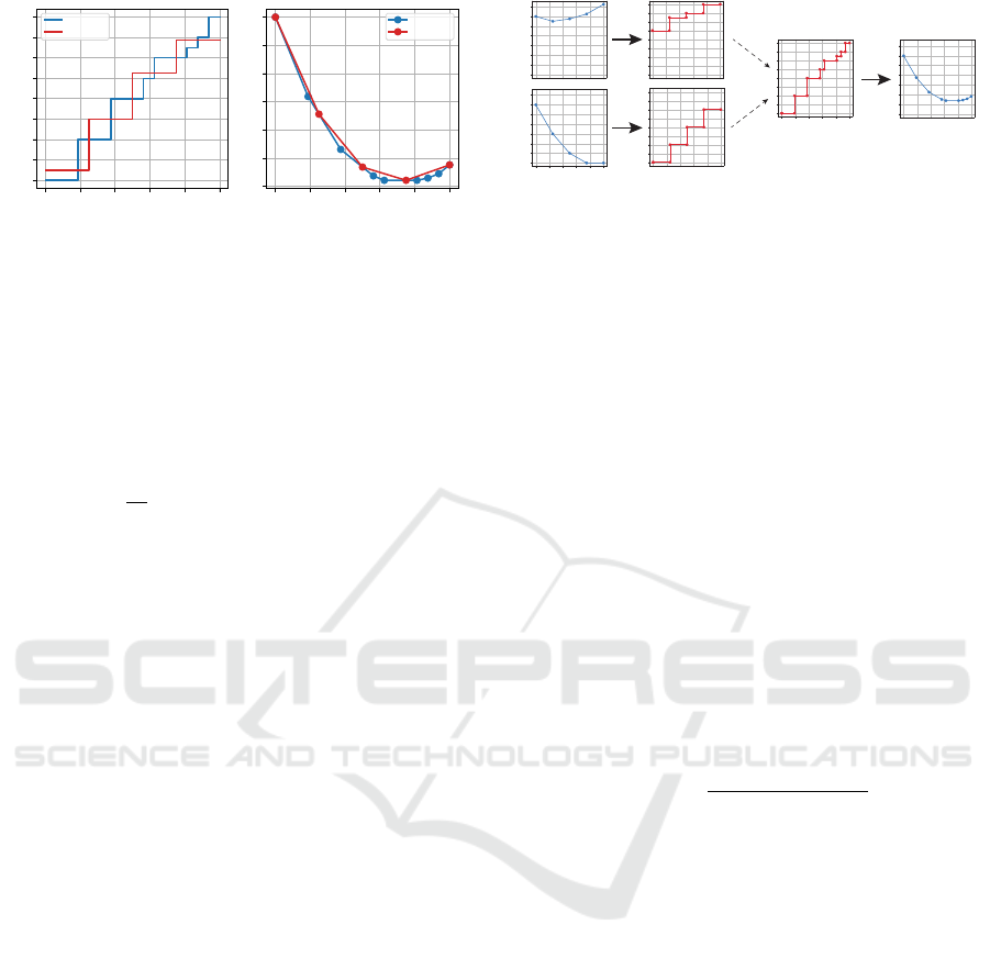
Lemma 1. Any discrete distribution has a piecewise

linear and convex yCVaR

function. Similarly, any

piecewise linear convex function can be seen as rep-

resenting a certain discrete distribution.

Particularly, the integral of the quantile function is the

Risk-averse Distributional Reinforcement Learning: A CVaR Optimization Approach

415

0.0 0.2 0.4 0.6 0.8 1.0

−3.0

−2.5

−2.0

−1.5

−1.0

−0.5

0.0

0.5

1.0

Quantile function

Exact

CVaR VI

0.0 0.2 0 .4 0.6 0.8 1.0

−1.2

−1.0

−0.8

−0.6

−0.4

−0.2

0.0

y CVaR

Exact

CVaR VI

Figure 1: Comparison of a discrete distribution and its ap-

proximation according to the CVaR linear interpolation op-

erator.

yCVaR

function

yCVaR

(Z) =

VaR

(Z)dβ (15)

and the derivative of the yCVaR

function is the quan-

tile function

∂

∂y

yCVaR

(Z) = VaR

(Z) (16)

3.1 CVaR Computation via Quantile

Representation

We propose the following procedure: instead of using

linear programming for the CVaR computation, we

use Lemma 1 and the underlying distributions repre-

sented by the yCVaR

function to compute CVaR at

each atom. The general steps of the computation are:

1. Transform yCVaR

(Z(x

)) of each reachable state

to a discrete probability distribution using (16).

2. Combine these to to a distribution representing the

full state-action distribution

3. Compute yCVaR

for all atoms using (15)

See Figure 2 for a visualization of the procedure.

Note that this procedure is linear (in number of tran-

sitions and atoms) for discrete distributions. The only

nonlinear step in the procedure is the sorting step in

mixing distributions. Since the values are pre-sorted

for each state x

, this is equivalent to a single step of

the Merge sort algorithm, which means it is also linear

in the number of atoms.

We show the explicit computation of the proce-

dure for linearly interpolated atoms in Algorithm 1 in

the bonus materials.

To show the correctness of this approach, we for-

mulate it as a solution to problem (11) in the next

paragraphs. Note that we skip the reward and gamma

scaling for readability’s sake. Extension to the Bell-

man operator is trivial.

Figure 2: Visualization of the CVaR computation for a sin-

gle state and action with two transition states. Thick arrows

represent the conversion between yCVaR

and the quantile

function.

3.2 ξ-computation

Similarly to Theorem 5 in (Chow et al., 2015), we

need a way to compute the y

t+1

= y

∗

) to ex-

tract the optimal policy. We compute ξ

∗

) by us-

ing the following intuition: y

t+1

represents portion of

the tail of Z(x

t+1

) that has values present in the com-

putation of CVaR

(Z(x

)). In the continuous case,

it is the probability in Z(x

t+1

) of values less than

VaR

(Z(x

)) as we show below.

Theorem 1. Let x

be only two states reachable

from state x via action a in a single transition. Let the

cumulative distribution functions of the state’s under-

lying distributions Z(x

),Z(x

) be strictly increasing

with unbounded support. Then the solution to mini-

mization problem (11) can be computed for i = 1,2

by setting

ξ(x

) =

Z(x

)



−1

Z(x,a)

(α)



(17)

The theorem is straightforwardly extendable to

multiple states by induction.

4 CVaR Q-LEARNING

While value iteration is a useful algorithm, it only

works when we have complete knowledge of the

environment - including the probability transitions

p(x

|x,a). This is often not the case in practice and

we have to rely on different methods, based on direct

interaction with the environment. One such algorithm

is the well-known Q-learning (Watkins and Dayan,

1992) that works by repeatedly updating the action

value estimate according to the sampled rewards and

states using a moving exponential average.

As a next contribution, we formulate a Q-learning

like algorithm for CVaR.

NCTA 2019 - 11th International Conference on Neural Computation Theory and Applications

416

4.1 CVaR Estimation

Before formulating a CVaR version of Q-learning, we

must ﬁrst talk about simply estimating CVaR, as it is

not as straightforward as the estimation of expected

value.

Given the primal deﬁnition of CVaR (3), if we

knew the exact s

∗

= VaR

, we could estimate the

CVaR as a simple expectation of the

(Z − s

∗

)

−

+ s

∗

function. As we do not know this value in advance, a

common approach is to ﬁrst approximate VaR

from

data, then use this estimate to compute its CVaR

This is usually done with a full data vector, requiring

the whole data history to be saved in memory.

When dealing with reinforcement learning, we

would like to store our current estimate as a scalar

instead. This requires ﬁnding a recursive expression

whose expectation is the CVaR value. Fortunately,

similar methods have been thoroughly investigated in

the stochastic approximation literature by (Robbins

and Monro, 1951).

The Robbins Monroe theorem has also been ap-

plied directly to CVaR estimation by (Bardou et al.,

2009), who used it to formulate a recursive impor-

tance sampling procedure useful for estimating CVaR

of long-tailed distributions.

First let us describe the method for one step esti-

mation, meaning we sample values (or rewards in our

case) r from some distribution and our goal is to esti-

mate CVaR

. The procedure requires us to maintain

two separate estimates V and C, being our VaR and

CVaR estimates respectively.

t+1

= V

+ β



1 −

≥r)



(18)

t+1

= (1 − β

+ β



(r −V

)

−



(19)

represents the learning rate at time t. An observant

reader may recognize a standard equation for quan-

tile estimation in equation (18) (see e.g. (Koenker

and Hallock, 2001) for more information on quan-

tile estimation/regression). The expectation of the up-

date



1 −

≥r)



is the inverse gradient of the

CVaR primal deﬁnition, so we are in fact performing

a Stochastic Gradient Descent on the primal.

Equation (19) then represents the moving expo-

nential average of the primal CVaR deﬁnition (3). The

estimations are proven to converge, given the usual re-

quirements on the learning rate (Bardou et al., 2009).

4.2 CVaR Q-learning

We ﬁrst deﬁne two separate values for each state, ac-

tion, and atom V,C : X ×A × Y → R where C(x,a,y)

represents CVaR

(Z(x, a)) of the distribution

, sim-

ilar to the deﬁnition (12). V (x, a,y) represents the

VaR

estimate, i.e. the estimate of the y−quantile of

a distribution recovered from CVaR

by Lemma 1.

A key to any temporal difference (TD) algorithm

is its update rule. The CVaR TD update rule extends

the improved value iteration procedure and we present

the full rule for uniform atoms in Algorithm 1.

Let us now go through the algorithm step by step.

We ﬁrst construct a new CVaR (line 3), representing

CVaR

(Z(x

)), by greedily selecting actions that yield

the highest CVaR for each atom.

The new values C(x

•

) are then transformed to the

underlying distribution (line 5) d and used to create

the target T d = r + γd. A natural Monte Carlo ap-

proach would be then to generate samples from this

target distribution and use these to update our esti-

mates V,C.

Since we know the target distributions exactly, we

do not have to actually sample; instead we use the

quantile values proportionally to their probabilities (in

the uniform case, this means exactly once) and apply

the respective VaR and CVaR update rules (lines 7, 8).

Algorithm 1: CVaR TD update.

1: input: x, a,x

2: for each i do

3: C(x

) = max

C(x

)

4: end for

5: d = extractDistribution(C(x

•

),y)

6: for each i, j do

7: V (x,a, y

) =

V (x,a, y

) + β

1 −

(V (x,a,y

)≥r+γd

)

8: C(x, a,y

) = (1 − β)C(x,a, y

V (x,a, y

) +

(r + γd

−V (x, a,y

))

−

9: end for

If the atoms aren’t uniformly spaced (log-spaced

atoms are motivated by the error bounds of CVaR

Value Iteration), we have to perform basic importance

We can read (x,y) as extended state - combining the in-

formation about (i) environment and (ii) risk perception. In

this sense, the extension is similar to extended reinforce-

ment Q learning as described in (Obayashi et al., 2015)

where the new component expresses the expresses the emo-

tional state of the agent.

Extracts the underlying distribution from CVaR, see

Algorithm 1 in bonus materials.

Risk-averse Distributional Reinforcement Learning: A CVaR Optimization Approach

417

sampling when updating the estimates . In contrast

with the uniform version, we iterate only over the

atoms and perform a single update for the whole tar-

get by taking an expectation over the target distribu-

tion. This is done by replacing lines 7, 8 with

V (x,a, y

) = V (x,a,y

) + β



1 −

(V (x,a,y

)≥r+γd

)



C(x, a,y

) = (1 − β)C(x,a, y

+β



V (x,a, y

) +

(r + γd

−V (x, a,y

))

−



(20)

The explicit computation of the expectation term for

VaR would then look like



1 −

(V (x,a,y

)≥r+γd

)



∑



1 −

(V (x,a,y

)≥r+γd

)



where p

= y

− y

j−1

represents the probability of d

The CVaR update expectation is computed analogi-

cally.

4.3 VaR-based Policy Improvement

CVaR Q-learning helps us to ﬁnd the CVaR

function,

but does not help us with retrieving the optimal policy.

Below we formulate an algorithm that allows us to get

the optimal policy.

Let us assume that we have successfully con-

verged with distributional value iteration and have

available the return distributions of some stationary

policy for each state and action. Our next goal is to

ﬁnd a policy improvement algorithm that will mono-

tonically increase the CVaR

criterion for selected α.

Recall the primal deﬁnition of CVaR (3)

CVaR

(Z) = max





(Z − s)

−



+ s



Our goal (7) can then be rewritten as

max

CVaR

) = max

max



− s)

−



+ s

As mentioned earlier, the primal solution is equivalent

to VaR

(Z)

CVaR

(Z) = max





(Z − s)

−



+ s





(Z − VaR

(Z))

−



+ VaR

(Z)

The main idea of VaR-based policy improvement

is the following: If we knew the value s

∗

in advance,

we could simplify the problem to maximize only

max

CVaR

) = max



− s

∗

)

−



+ s

∗

(21)

Given that we have access to the return distribu-

tions, we can improve the policy by simply choos-

ing an action that maximizes CVaR

in the ﬁrst

state a

= argmax

CVaR

)), setting s

∗

VaR

(Z(x

)) and focus on maximization of the

simpler criterion.

This can be seen as coordinate ascent with the fol-

lowing phases:

1. Maximize

E [(Z

) − s)

−

] + s w.r.t. s while

keeping π ﬁxed. This is equivalent to computing

CVaR according to the primal.

2. Maximize

E [(Z

) − s)

−

] + s w.r.t. π while

keeping s ﬁxed. This is the policy improvement

step.

3. Recompute CVaR

∗

) where π

∗

is the new pol-

icy.

Since our goal is to optimize the criterion of the dis-

tribution starting at x

, we need to change the value

s while traversing the MDP (where we have only ac-

cess to Z(x

)). We do this by recursively updating the

s we maximize by setting s

t+1

− r

. See Algo-

rithm 2 for the full procedure which we justify in the

following theorem.

Algorithm 2: VaR-based policy improvement.

a = arg max

CVaR

(Z(x

,a))

s = VaR

(Z(x

,a))

Take action a, observe x,r

while x is not terminal do

s =

s − r

a = arg max

E [(Z(x,a) − s)

−

]

Take action a, observe x,r

end while

Theorem 2. Let π be a stationary policy, α ∈ (0,1].

By following policy π

∗

from algorithm 2, we improve

CVaR

(Z) in expectation:

CVaR

) ≤ CVaR

∗

)

Note that while the resulting policy is nonstation-

ary, we do not need an extended state-space to follow

this policy. It is only necessary to remember our pre-

vious value of s.

The ideas presented here were partially explored

by (B

auerle and Ott, 2011) although not to this extent.

See Remark 3.9 in (B

auerle and Ott, 2011) for details.

4.3.1 CVaR Q-learning Extension

We would now like to use the policy improvement al-

gorithm in order to extract the optimal policy from

NCTA 2019 - 11th International Conference on Neural Computation Theory and Applications

418

CVaR Q-learning. This would mean optimizing

E [(Z

− s)

−

] in each step. A problem we encounter

here is that we have access only to the discretized dis-

tributions and we cannot extract the values between

selected atoms.

To solve this, we propose an approximate heuris-

tic that uses linear interpolation to extract the VaR of

given distribution.

The expression E [(Z

− s)

−

] is computed by tak-

ing the expectation of the distribution before the value

s. We are therefore looking for value y where VaR

s. This value is linearly interpolated from VaR

i−1

and

VaR

where y

= min

{

y : VaR

≥ s

}

. The expecta-

tion is then taken over the extracted distribution, as

this is the distribution that approximates CVaR the

best.

See Algorithm 2 and Figure 1 in the bonus mate-

rials for more intuition behind the heuristic.

5 DEEP CVAR Q-LEARNING

A big disadvantage of value iteration and Q-learning

is the necessity to store a separate value for each state.

When the size of the state-space is too large, we are

unable to store the action-value representation and the

algorithms become intractable. To overcome this is-

sue, it is common to use function approximation to-

gether with Q-learning. (Mnih et al., 2015) proposed

the Deep Q-learning (DQN) algorithm and success-

fully trained on multiple different high-dimensional

environments, resulting in the ﬁrst artiﬁcial agent ca-

pable of learning a diverse array of challenging tasks.

In this section, we extend CVaR Q-learning to its

deep Q-learning variant and show the practicality and

scalability of the proposed methods.

The transition from CVaR Q-learning to Deep

CVaR Q-learning (CVaR DQN) follows the same

principles as the one from Q-learning to DQN. First

signiﬁcant change compared to DQN or QR-DQN

(Dabney et al., 2017) is that we need to represent two

separate values - one for V , one for C. As with DQN,

we need to reformulate the updates as arguments min-

imizing some loss function.

5.1 Loss Functions

The loss function for V (x,a,y) is similar to QR-DQN

loss in that we wish to ﬁnd quantiles of a particu-

lar distribution. The target distribution however is

constructed differently - in CVaR-DQN we extract

the distribution from the yCVaR

function of the next

state T V = r + γd.

VaR

∑

i=1

(r + γd

−V

(x,a))(y

−

(x,a)≥r+γd

)

(22)

where d

are atoms of the extracted distribution.

Constructing the CVaR loss function consists of

transforming the running mean into mean squared er-

ror, again with the transformed distribution atoms d

CVaR

∑

i=1



(x,a)+

(r + γd

−V

(x,a))

−

−C

(x,a)



(23)

Putting it all together, we are now able to construct

the full CVaR-DQN loss function.

L = L

VaR

+ L

CVaR

(24)

Combining the loss functions with the full DQN

algorithm, we get the full CVaR-DQN with experi-

ence replay

. Note that we utilize a target network C

that is used for extraction of the target values of C,

similarly to the original DQN. The network V does

not need a target network since the target is con-

structed independently of the value V .

6 EXPERIMENTS

6.1 CVaR Value Iteration

We test the proposed algorithm on the same task as

(Chow et al., 2015). The task of the agent is to navi-

gate on a rectangular grid to a given destination, mov-

ing in its four-neighborhood. To encourage fast move-

ment towards the goal, the agent is penalized for each

step by receiving a reward -1. A set of obstacles is

placed randomly on the grid and stepping on an ob-

stacle ends the episode while the agent receives a re-

ward of -40. To simulate sensing and control noise,

the agent has a δ = 0.05 probability of moving to a

different state than intended.

For our experiments, we choose a 40 × 60 grid-

world and approximate the αCVaR

function using

21 log-spaced atoms. The learned policies on a sam-

ple grid are shown in Figure 3.

See Algorithm 3 in the bonus materials.

All code is publicly available at https://bit.ly/

2YFCDyE

Risk-averse Distributional Reinforcement Learning: A CVaR Optimization Approach

419

While (Chow et al., 2015) report computation

time on the order of hours (using the highly optimized

CPLEX Optimizer), our naive Python implementation

converged under 20 minutes.

S G

α = 0.1

S G

α = 0.2

S G

α = 0.3

S G

α = 1.0

−30

−25

−20

−15

−10

−5

−25

−20

−15

−10

−5

−20

−15

−10

−5

−20.0

−17.5

−15.0

−12.5

−10.0

−7.5

−5.0

−2.5

0.0

Figure 3: Grid-world simulations. The optimal determinis-

tic paths are shown together with CVaR estimates for given

α.

6.2 CVaR Q-learning

We use the same gridworld for our experiments. Since

the positive reward is very sparse, we chose to run

CVaR Q-learning on a smaller environment of size

10 × 15. We trained the agent for 10,000 sampled

episodes with learning rate β = 0.4 that dropped each

10 episodes by a factor of 0.995. The used policy

was ε−greedy and maximized expected value (α = 1)

with ε = 0.5. Notice the high value of ε. We found

that lower ε values led to overﬁtting the optimal ex-

pected value policy as the agent updated states out of

the optimal path sparsely.

With said parameters, the agent was able to learn

the optimal policies for different levels of α. See

Figure 4 for learned policies and Figure 5 for Monte

Carlo comparisons.

S G

α = 0.1

S G

α = 0.3

S G

α = 0.6

S G

α = 1.0

−35

−30

−25

−20

−15

−10

−5

−20.0

−17.5

−15.0

−12.5

−10.0

−7.5

−5.0

−2.5

0. 0

−20.0

−17.5

−15.0

−12.5

−10.0

−7.5

−5.0

−2.5

0.0

−14

−12

−10

−8

−6

−4

−2

Figure 4: Grid-world Q-learning simulations. The optimal

deterministic paths are shown together with CVaR estimates

for given α.

−60 −50 −40 −30 −20

0.00

0.05

0.10

0.15

0.20

0.25

Q-learning

CVaR Q-learning

Figure 5: Histograms from 10000 runs generated by Q-

learning and CVaR Q-learning with α = 0.1.

6.3 Deep CVaR Q-learning

To test the approach in a complex setting, we applied

the CVaR DQN algorithm to environments with vi-

sual state representation, which would be intractable

for Q-learning without approximation.

6.3.1 Ice Lake

Ice Lake is a visual environment speciﬁcally designed

for risk-sensitive decision making. Imagine you are

standing on an ice lake and you want to travel fast to a

point on the lake. Will you take the a shortcut and risk

falling into the cold water or will you be more patient

and go around? This is the basic premise of the Ice

Lake environment which is visualized in Figure 6.

The agent has ﬁve discrete actions, namely go

Left, Right, Up, Down and Noop. These correspond

to moving in the respective directions or no operation.

Since the agent is on ice, there is a sliding element

in the movement - this is mainly done to introduce

time dependency and makes the environment a little

harder. The environment is updated thirty times per

second.

The agent receives a negative reward of -1 per sec-

ond, the episode ends with reward 100 if he reaches

the goal unharmed or -50 if the ice breaks. This par-

ticular choice of reward leads to about a 15% chance

of breaking the ice when taking the shortcut and it is

still advantageous for a risk-neutral agent to take the

dangerous path.

6.3.2 Network Architecture

During our experiments we used a simple Multi-

Layered Perceptron with 64 hidden units for a base-

line experiment and later the original DQN architec-

ture with a visual representation. In our baseline ex-

periments, the state was represented with x- y- posi-

tion and velocity.

The architecture used in our experiments differs

slightly from the original one used in DQN. In our

NCTA 2019 - 11th International Conference on Neural Computation Theory and Applications

420

Figure 6: The Ice Lake environment. The agent is black and

his target is green. The blue ring represents a dangerous

area with risk of breaking the ice. Grey arrow shows the

optimal risk-neutral path, red shows the risk-averse path.

case the output is not a single value but instead a vec-

tor of values for each action, representing CVaR

VaR

for the different conﬁdence levels y. This issue

is reconciled by having the output of shape |A| × N

where N is the number of atoms we want to use and

|A| is the action space size.

Another important difference is that we must work

with two outputs - one for C, one for V . We have ex-

perimented with two separate networks (one for each

value) and also with a single network differing only

in the last layer. This approach may be advantageous,

since we can imagine that the information required

for outputting correct V or C is similar. Furthermore,

having a single network instead of two eases the com-

putation requirements.

We tested both approaches and since we didn’t

ﬁnd signiﬁcant performance differences, we settled

on the faster version with shared weights. We also

used 256 units instead of 512 to ease the computation

requirements and used Adam (Kingma and Ba, 2014)

as the optimization algorithm.

The implementation was done in Python and the

neural networks were built using Tensorﬂow (Abadi

et al., 2016) as the framework of choice for gradient

descent. The code was based on OpenAi baselines

(Dhariwal et al., 2017), an open-source DQN imple-

mentation.

6.3.3 Parameter Tuning

During our experiments, we tested mostly with α = 1

so as to ﬁnd reasonable policies quickly. We noticed

that the optimal policy with respect to expected value

was found fast and other policies were quickly aban-

doned due to the character of ε-greedy exploration.

Unlike standard Reinforcement Learning, the CVaR

optimization approach requires to ﬁnd not one but in

fact a continuous spectrum of policies - one for each

possible α. This fact, together with the exploration-

exploitation dilemma, contributes to the difﬁculty of

learning the correct policies.

After some experimentation, we settled on the fol-

lowing points:

• The training beneﬁts from a higher value of ε than

DQN. We settled on 0.3 as a reasonable value

with the ability to explore faster, while making the

learned trajectories exploitable.

• Training with a single policy is insufﬁcient in

larger environments. Instead of maximizing

CVaR for α = 1 as in our CVaR Q-learning ex-

periments, we change the value α randomly for

each episode (uniformly over (0,1]).

• The random initialization used in deep learning

has a detrimental effect on the initial distribution

estimates, due to the way how the target is con-

structed and this sometimes leads to the introduc-

tion of extreme values during the initial training.

We have found that clipping the gradient norm

helps to mitigate these problems and overall helps

with the stability of learning.

6.3.4 Results

With the tweaked parameters, both versions (baseline

and visual) were able to converge and learned both the

optimal expected value policy and the risk-sensitive

policy, as in Figure 6

Although we tested with the vanilla version of

DQN, we expect that all the DQN improvements such

as experience replay (Hessel et al., 2017), dueling

(Wang et al., 2015), parameter noise (Plappert et al.,

2017) and others (combining the improvements mat-

ters, see (Hessel et al., 2017)) should have a positive

effect on the learning performance. Another practical

improvement may be the introduction of Huber loss,

similarly to QR-DQN.

7 CONCLUSION

In this paper, we tackled the problem of dynamic

risk-averse reinforcement learning. Speciﬁcally we

focused on optimizing the Conditional Value-at-Risk

objective.

The work mainly builds on the CVaR Value Iter-

ation algorithm (Chow et al., 2015), a dynamic pro-

gramming method for solving CVaR MDPs.

Our ﬁrst original contribution is the proposal of a

different computation procedure for CVaR value iter-

ation. The novel procedure reduces the computation

time from polynomial to linear. More speciﬁcally, our

approach does not require solving a series of Linear

See videos in the bonus materials.

Risk-averse Distributional Reinforcement Learning: A CVaR Optimization Approach

421

Programs and instead ﬁnds solutions to the internal

optimization problems in linear time by appealing to

the underlying distributions of the CVaR function. We

formally proved the correctness of our solution for a

subset of probability distributions.

Next we proposed a new sampling algorithm we

call CVaR Q-learning, that builds on our previous re-

sults. Since the algorithm is sample-based, it does

not require perfect knowledge of the environment.

In addition, we proposed a new policy improvement

algorithm for distributional reinforcement learning,

proved its correctness and later used it as a heuris-

tic for extracting the optimal policy from CVaR Q-

learning. We empirically veriﬁed the practicality of

the approach and our agent is able to learn multiple

risk-sensitive policies all at once.

To show the scalability of the new algorithm, we

extended CVaR Q-learning to its approximate variant

by formulating the Deep CVaR loss function and used

it in a deep learning context. The new Deep CVaR

Q-learning algorithm is able to learn different risk-

sensitive policies from raw pixels.

We believe that the CVaR objective is a practical

framework for computing control policies that are ro-

bust with respect to both stochasticity and model per-

turbations. Collectively, our work enhances the cur-

rent state-of-the-art methods for CVaR MDPs and im-

proves both practicality and scalability of the avail-

able approaches.

7.1 Future Work

Our contributions leave several pathways open for fu-

ture work. Firstly, our proof of the improved CVaR

Value Iteration works only for a subset of proba-

bility distributions and it shall be at least theoreti-

cally beneﬁcial to prove the same for general distri-

bution. The result may also be necessary for the con-

vergence proof of CVaR Q-learning. Another miss-

ing piece required for proving the asymptotic conver-

gence of CVaR Q-learning is the convergence of re-

cursive CVaR estimation. Currently the convergence

has been proven only for continuous distributions and

more general proof is required to show the CVaR Q-

learning convergence.

We also highlighted a way of extracting the cur-

rent policy from converged CVaR Q-learning values.

While the method is consistent in the limit, for prac-

tical purposes it serves only as a heuristic. It remains

to be seen if there are better, perhaps exact ways of

extracting the optimal policy.

The work of (B

auerle and Ott, 2011) shares a con-

nection with CVaR Value Iteration and may be of

practical use for CVaR MDPs. The relationship be-

tween CVaR Value Iteration and Bauerle’s work is

very similar to the c51 algorithm (Bellemare et al.,

2017) and QR-DQN (Dabney et al., 2017). Bauerle’s

work is also a certain ’transposition’ of CVaR Value

Iteration and a comparison between the two may be

beneﬁcial. Of particular interest is the ease of extract-

ing the optimal policy in a sampling version of the

algorithm.

Lastly, our experimental work focused mostly on

toy problems that demonstrated the basic function-

ality of the proposed algorithms. Since we believe

our methods are practical beyond these toy settings,

we would like to apply the techniques on relevant

problems from the ﬁnancial sector and on practical

robotics, and other risk-sensitive applications, includ-

ing interdisciplinary reasearch on emotional percep-

tion of risk (Obayashi et al., 2015).

REFERENCES

Abadi, M., Barham, P., Chen, J., Chen, Z., Davis, A., Dean,

J., Devin, M., Ghemawat, S., Irving, G., Isard, M.,

et al. (2016). Tensorﬂow: A system for large-scale

machine learning. In OSDI, volume 16, pages 265–

283.

Bahdanau, D., Cho, K., and Bengio, Y. (2014). Neural ma-

chine translation by jointly learning to align and trans-

late. arXiv preprint arXiv:1409.0473.

Bardou, O., Frikha, N., and Pages, G. (2009). Recursive

computation of value-at-risk and conditional value-at-

risk using mc and qmc. In Monte Carlo and quasi-

Monte Carlo methods 2008, pages 193–208. Springer.

auerle, N. and Ott, J. (2011). Markov decision pro-

cesses with average-value-at-risk criteria. Mathemati-

cal Methods of Operations Research, 74(3):361–379.

Bellemare, M. G., Dabney, W., and Munos, R. (2017). A

distributional perspective on reinforcement learning.

arXiv preprint arXiv:1707.06887.

Bellman, R. (1957). A markovian decision process. Journal

of Mathematics and Mechanics, pages 679–684.

Chow, Y., Tamar, A., Mannor, S., and Pavone, M. (2015).

Risk-sensitive and robust decision-making: a cvar op-

timization approach. In Advances in Neural Informa-

tion Processing Systems, pages 1522–1530.

Committee, B. et al. (2013). Fundamental review of the

trading book: A revised market risk framework. Con-

sultative Document, October.

Coraluppi, S. P. (1998). Optimal control of markov decision

processes for performance and robustness.

Dabney, W., Ostrovski, G., Silver, D., and Munos, R.

(2018). Implicit quantile networks for distributional

reinforcement learning.

Dabney, W., Rowland, M., Bellemare, M. G., and Munos,

R. (2017). Distributional reinforcement learning with

quantile regression. arXiv preprint arXiv:1710.10044.

NCTA 2019 - 11th International Conference on Neural Computation Theory and Applications

422

Dhariwal, P., Hesse, C., Klimov, O., Nichol, A., Plappert,

M., Radford, A., Schulman, J., Sidor, S., and Wu, Y.

(2017). Openai baselines. https://github.com/openai/

baselines.

Garcıa, J. and Fern

andez, F. (2015). A comprehensive sur-

vey on safe reinforcement learning. Journal of Ma-

chine Learning Research, 16(1):1437–1480.

Hamid, O. and Braun, J. (2019). Reinforcement Learning

and Attractor Neural Network Models of Associative

Learning, pages 327–349.

Hessel, M., Modayil, J., Van Hasselt, H., Schaul, T., Ostro-

vski, G., Dabney, W., Horgan, D., Piot, B., Azar, M.,

and Silver, D. (2017). Rainbow: Combining improve-

ments in deep reinforcement learning. arXiv preprint

arXiv:1710.02298.

Howard, R. A. and Matheson, J. E. (1972). Risk-sensitive

markov decision processes. Management science,

18(7):356–369.

Kingma, D. P. and Ba, J. (2014). Adam: A

method for stochastic optimization. arXiv preprint

arXiv:1412.6980.

Koenker, R. and Hallock, K. F. (2001). Quantile regression.

Journal of economic perspectives, 15(4):143–156.

Krizhevsky, A., Sutskever, I., and Hinton, G. E. (2012). Im-

agenet classiﬁcation with deep convolutional neural

networks. In Advances in neural information process-

ing systems, pages 1097–1105.

Leike, J., Martic, M., Krakovna, V., Ortega, P. A., Everitt,

T., Lefrancq, A., Orseau, L., and Legg, S. (2017). Ai

safety gridworlds. arXiv preprint arXiv:1711.09883.

Lesser, K. and Abate, A. (2017). Multi-objective optimal

control with safety as a priority. In 2017 ACM/IEEE

8th International Conference on Cyber-Physical Sys-

tems (ICCPS), pages 25–36.

Macek, K. (2010). Predictive control via lazy learning and

stochastic optimization. In Doktorandsk

e dny 2010 -

Sborn

ık doktorand

u FJFI, pages 115–122.

Majumdar, A. and Pavone, M. (2017). How should a robot

assess risk? towards an axiomatic theory of risk in

robotics. arXiv preprint arXiv:1710.11040.

Miller, C. W. and Yang, I. (2017). Optimal control of condi-

tional value-at-risk in continuous time. SIAM Journal

on Control and Optimization, 55(2):856–884.

Mnih, V., Kavukcuoglu, K., Silver, D., Rusu, A. A., Veness,

J., Bellemare, M. G., Graves, A., Riedmiller, M., Fid-

jeland, A. K., Ostrovski, G., et al. (2015). Human-

level control through deep reinforcement learning.

Nature, 518(7540):529.

Morimura, T., Sugiyama, M., Kashima, H., Hachiya, H.,

and Tanaka, T. (2012). Parametric return density es-

timation for reinforcement learning. arXiv preprint

arXiv:1203.3497.

Obayashi, M., Uto, S., Kuremoto, T., Mabu, S., and

Kobayashi, K. (2015). An extended q learning sys-

tem with emotion state to make up an agent with indi-

viduality. 2015 7th International Joint Conference on

Computational Intelligence (IJCCI), 3:70–78.

Pﬂug, G. C. and Pichler, A. (2016). Time-consistent de-

cisions and temporal decomposition of coherent risk

functionals. Mathematics of Operations Research,

41(2):682–699.

Plappert, M., Houthooft, R., Dhariwal, P., Sidor, S.,

Chen, R. Y., Chen, X., Asfour, T., Abbeel, P., and

Andrychowicz, M. (2017). Parameter space noise for

exploration. arXiv preprint arXiv:1706.01905.

Prashanth, L. (2014). Policy gradients for cvar-constrained

mdps. In International Conference on Algorithmic

Learning Theory, pages 155–169. Springer.

Robbins, H. and Monro, S. (1951). A stochastic approxi-

mation method. The annals of mathematical statistics,

pages 400–407.

Rockafellar, R. T. and Uryasev, S. (2000). Optimization of

conditional value-at-risk. Journal of risk, 2:21–42.

Silver, D., Schrittwieser, J., Simonyan, K., Antonoglou, I.,

Huang, A., Guez, A., Hubert, T., Baker, L., Lai, M.,

Bolton, A., et al. (2017). Mastering the game of go

without human knowledge. Nature, 550(7676):354.

Sobel, M. J. (1982). The variance of discounted markov

decision processes. Journal of Applied Probability,

19(4):794–802.

Sutton, R. S. and Barto, A. G. (1998). Reinforcement learn-

ing: An introduction, volume 1. MIT press Cam-

bridge.

Tamar, A., Chow, Y., Ghavamzadeh, M., and Mannor,

S. (2017). Sequential decision making with coher-

ent risk. IEEE Transactions on Automatic Control,

62(7):3323–3338.

Tamar, A., Glassner, Y., and Mannor, S. (2015). Optimizing

the cvar via sampling. In AAAI, pages 2993–2999.

Wang, Z., Schaul, T., Hessel, M., Van Hasselt, H., Lanc-

tot, M., and De Freitas, N. (2015). Dueling network

architectures for deep reinforcement learning. arXiv

preprint arXiv:1511.06581.

Watkins, C. J. and Dayan, P. (1992). Q-learning. Machine

learning, 8(3-4):279–292.

Risk-averse Distributional Reinforcement Learning: A CVaR Optimization Approach

423