
Modified Differential Evolution in the Load Balancing Problem for the
iFDAQ of the COMPASS Experiment at CERN
Ond
ˇ
rej
ˇ
Subrt
1
, Martin Bodl
´
ak
2
, Matou
ˇ
s Jandek
1
, Vladim
´
ır Jar
´
y
1
, Anton
´
ın Kv
ˇ
eto
ˇ
n
2
, Josef Nov
´
y
1
,
Jan Tomsa
1
and Miroslav Virius
1
1
Czech Technical University in Prague, Prague, Czech Republic
2
Charles University, Prague, Czech Republic
Keywords:
Data Acquisition System, Differential Evolution, Genetic Algorithm, Load Balancing, Optimization.
Abstract:
In general, state-of-the-art data acquisition systems in high energy physics experiments must satisfy high re-
quirements in terms of reliability, efficiency and data rate capability. The paper introduces the Load Balancing
(LB) problem of the intelligent, FPGA-based Data Acquisition System (iFDAQ) of the COMPASS experi-
ment at CERN and proposes a solution based on genetic algorithms. Since the LB problem is N P -complete,
it challenges analytical and heuristic methods in finding optimal solutions in reasonable time. Differential
Evolution (DE) is a type of evolutionary algorithms, which has been used in many optimization problems due
to its simplicity and efficiency. Therefore, the Modified Differential Evolution (MDE) is inspired by DE and
is presented in more detail. The MDE algorithm has newly-designed crossover and mutation operator and its
selection mechanism is inspired by Simulated Annealing (SA). Moreover, the proposal uses an adaptive scal-
ing factor and recombination rate affecting the exploration and exploitation of the MDE algorithm. Thus, the
MDE represents a new efficient stochastic search technique for the LB problem. The proposed MDE algorithm
is examined on two LB test cases and compared with other LB solution methods.
1 INTRODUCTION
The intelligent, FPGA-based Data Acquisition Sys-
tem (iFDAQ) (Bodlak et al., 2016; Bodlak et al.,
2014) reads out data from the detectors of the COM-
PASS (COmmon Muon Proton Apparatus for Struc-
ture and Spectroscopy) experiment (Alexakhin et al.,
2010) being a high-energy particle physics experi-
ment with fixed-target situated on the M2 beamline of
the Super Proton Synchrotron (SPS) particle acceler-
ator at the CERN laboratory in Geneva, Switzerland.
In complex readout data systems, such as the iF-
DAQ, the data streams must be properly allocated in
order for the load to be well-balanced in the system
(Kameda et al., 1997). Thus, the necessity of solving
the Load Balancing (LB) problem arises.
The paper is organized as follows. Firstly, the LB
problem is introduced in Section 2. Subsection 2.1
gives the proper definition of the LB problem. Com-
plexity of the LB problem is proved in Subsection 2.2.
Secondly, Section 3 describes the proposal of the
Modified Differential Evolution (MDE) algorithm be-
ing applicable to the LB problem. All parts of the
MDE algorithm are discussed in an extensive way.
Finally, numerical results are stated in Section 4
to demonstrate how the MDE approach is successful
and efficient in solving the LB problem. Then, the
results acquired by the MDE are compared with other
LB solution methods.
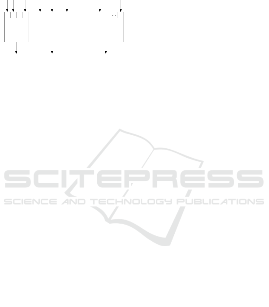
2 LOAD BALANCING PROBLEM
For the iFDAQ, the most challenging task from the
LB point of view is load balancing at the multiplexer
(MUX) level. The optimization criterion is mini-
mization of the difference between the output flows
of the individual multiplexers. This minimization is
achieved by remapping the connection of inputs to
input ports of the multiplexers. Each input port es-
tablishes a connection between a data source (a de-
tector or a data concentrator) and the MUX level. For
the COMPASS experiment, it is necessary to consider
flows varying from 0 B to 10 kB for each input port.
In Figure 1, a visualization of LB at the MUX
level is given. There are m MUXes with p ingoing
ports each. Moreover, n ∈ N flows f
k
1
, f
k
2
,..., f
k
mp
∈
Šubrt, O., Bodlák, M., Jandek, M., Jarý, V., Kv
ˇ
eto
ˇ
n, A., Nový, J., Tomsa, J. and Virius, M.
Modified Differential Evolution in the Load Balancing Problem for the iFDAQ of the COMPASS Experiment at CERN.
DOI: 10.5220/0008319102130220
In Proceedings of the 11th International Joint Conference on Computational Intelligence (IJCCI 2019), pages 213-220
ISBN: 978-989-758-384-1
Copyright
c
2019 by SCITEPRESS – Science and Technology Publications, Lda. All rights reserved
213
2
p
p + 1
p + 2
2p
1
MUX
1
MUX
2
MUX
m
(m − 1)p + 1
mp
f
k
1
f
k
2
f
k
p
f
k
p+1
f
k
p+2
f
k
2p
f
k
(m−1)p+1
f
k
mp
p
X
i=1
f
k
i
2p
X
i=p+1
f
k
i
mp
X
i=(m−1)p+1
f
k
i
Figure 1: Visualization of LB at the MUX level.
N
0
, where n = m · p, are shown in the figure with in-
dices k
1
,k
2
,. . .,k
mp
∈ {i | 1 ≤ i ≤ n} ∧ ∀i, j : k
i
6= k
j
.
Despite the fact that each flow varies from 0 B
to 10 kB in the COMPASS experiment, the domain
N
0
is used. The motivation comes from a general ap-
proach to LB. Moreover, a flow with 0 B can be either
a physical connected input port sending no data or an
empty input port where no data source is connected
to. In brief, there are always n = m · p flows regard-
less whether all ports are used or not.
2.1 Problem Formulation
This subsection deals with a proper definition of the
LB problem and preparation for discussion of the
complexity of the LB problem. The Multiple Knap-
sack (MK) problem (Kellerer et al., 2004) is useful
for the examination of the LB problem complexity as
it can be shown that there exists a polynomial reduc-
tion from the MK problem to the LB problem. As MK
problem is N P -complete, this implies the LB prob-
lem is N P -complete.
Definition 1. Let m ∈ N denote the number of MUXes
with p ∈ N ingoing ports each, i.e., n = m · p ∈ N
ingoing ports in total and flows f
1
, f
2
,. . ., f
n
∈ N
0
.
Let S
1
,S
2
,. . .,S
m
be subsets of indices and F =
&
n
∑
i=1
f
i
/m
'
be a theoretical average flow for one
MUX. The Load Balancing (LB) problem is an op-
timization problem such that:
To minimize
v
u
u
t
m
∑
i=1
F −
∑
j∈S
i
f
j
!
2
, (1)
subject to the constraints
• each flow must be allocated
m
[
i=1
S
i
= {i | i ∈ 1,... ,n} (2)
• each flow must be allocated at most once
S
i
∩ S
j
=
/
0 ∀i, j = 1,..., m ∧ i 6= j (3)
• each MUX has p ports
|S
i
| = p ∀i = 1, . .., m (4)
Being a generalization of the well-known Knap-
sack problem (Kellerer et al., 2004), the MK problem
represents an extension to m knapsacks.
Definition 2. Given n ∈ N items with weights
w
1
,w
2
,. . .,w
n
∈ N and values v
1
,v
2
,. . .,v
n
∈ R
+
, and
m ∈ N knapsacks with capacities W
1
,W
2
,. . .,W
m
∈ N.
The Multiple Knapsack (MK) problem is an optimiza-
tion problem such that:
To maximize
m
∑
i=1
n
∑
j=1
v
j
x
i j
, (5)
subject to the constraints
• maximum knapsack capacity
n
∑
j=1
w
j
x
i j
≤ W
i
∀i = 1,... ,m (6)
• each item must be allocated at most once
m
∑
i=1
x
i j
≤ 1 ∀ j = 1,... ,n (7)
• assignment of item
x
i j
∈ {0,1} ∀i = 1, . .., m, ∀ j = 1,..., n (8)
2.2 Problem Complexity
The Knapsack problem is N P -complete (Kellerer
et al., 2004). Being a generalization of the Knapsack
problem, the MK problem is N P -complete.
In order to determine the complexity of the LB
problem, the decision version of the LB problem must
be defined at first: Are there subsets S
1
,S
2
,. . .,S
m
such that
m
[
i=1
S
i
= {i | i ∈ 1,. . .,n} and S
i
∩ S
j
=
/
0,∀i, j = 1,. . .,m ∧ i 6= j and |S
i
| = p, ∀i = 1,... ,m
and
∑
j∈S
i
f
j
≤ F,∀i = 1, ..., m, where F =
&
n
∑
i=1
f
i
/m
'
?
Theorem 1. The Load Balancing (LB) problem is
N P -complete.
Proof. First, the LB problem is a N P problem. The
proof are the subsets S
1
,S
2
,. . .,S
m
of flow indices that
are chosen and the verification process is to compute
|S
i
| = p,∀i = 1,. ..,m and
∑
j∈S
i
f
j
≤ F,∀i = 1,... ,m,
which takes polynomial time in the size of input.
ECTA 2019 - 11th International Conference on Evolutionary Computation Theory and Applications
214

Second, it will be shown there is a polynomial re-
duction from the MK problem to the LB problem. It
suffices to show that there exists a polynomial time
reduction Q(·) such that Q(x) is a YES instance to the
LB problem iff x is a YES instance to the MK prob-
lem. Suppose there are given f
1
, f
2
,. . ., f
n
, for the LB
problem, consider the following MK problem: W
i
=
F,V
i
= p,∀i = 1, . .., m and w
i
= f
i
,v
i
= 1 + f
i
/h,∀i =
1,. . .,n, where h >
n
∑
i=1
f
i
and K =
m
[
i=1
K
i
⊆ {1,..., n}
and K
i
∩K
j
=
/
0,∀i, j = 1,. ..,m ∧i 6= j, where K
i
rep-
resents indices of items assigned to the i-th knapsack.
Here, Q(·) is the process converting the MK problem
to the LB problem. It is clear that this process is poly-
nomial in the input size.
If x is a YES instance for the MK prob-
lem, with the chosen sets K
1
,K
2
,. . .,K
m
, let R =
{1,. . .,n}\
m
[
i=1
K
i
. It follows that
∑
j∈K
i
w
j
=
∑
j∈K
i
f
j
≤
W
i
= F,∀i = 1,... ,m and it remains to prove there are
p items in each knapsack. It follows that
∑
j∈K
i
v
j
=
∑
j∈K
i
(1 + f
j
/h) ≥ V
i
= p,∀i = 1,. .., m and thus, there
must be at least p items in each knapsack to satisfy
the inequality. Moreover, n = m · p implies there must
be exactly p items in each knapsack and thus, R =
/
0.
Therefore, the sets K
1
,K
2
,. . .,K
m
correspond to sets
S
1
,S
2
,. . .,S
m
, respectively, and x is a YES instance
for the LB problem.
Conversely, if Q(x) is a YES instance for the
LB problem, there exists S
1
,S
2
,. . .,S
m
such that S
i
∩
S
j
=
/
0,∀i, j = 1, . .., m ∧ i 6= j and
m
[
i=1
S
i
= {i | i ∈
1,. . .,n} and |S
i
| = p,∀i = 1, ..., m and
∑
j∈S
i
f
j
≤
F,∀i = 1, . .., m. Let the MK problem consist of m
knapsacks and let the i-th knapsack contain the items
corresponding to indices in S
i
, and it follows that
∑
j∈K
i
w
j
=
∑
j∈K
i
f
j
≤ W
i
= F, ∀i = 1,. ..,m and
∑
j∈K
i
v
j
=
∑
j∈K
i
(1 + f
j
/h) ≥ V
i
= p, ∀i = 1,... ,m. Therefore,
Q(x) is a YES instance for the MK problem.
This proves the N P -completeness of the LB
problem.
3 MODIFIED DIFFERENTIAL
EVOLUTION
Belonging to the Evolutionary Algorithms (EA) class
(Eiben and Smith, 2015), a Genetic Algorithm (GA)
(Affenzeller et al., 2018) is a heuristic technique in-
spired by the process of natural selection and evolu-
tionary biology. It attempts to simulate evolutionary
principles in order to find estimate solutions of opti-
mization problems. These algorithms use techniques
and strategies simulating processes well-known from
nature – heredity, mutation, natural selection and
crossover.
The main principle of the GA process is grad-
ual production of stronger generations containing in-
dividuals representing different solutions of a prob-
lem. An individual is represented by the vector x =
(x
1
,x
2
,. . .,x
n
)
T
. In the optimization process, a new
population is created in each generation and each in-
dividual in a population represents just one solution
of a problem. As the population evolves, solutions
improve.
Differential Evolution (DE) (Storn and Price,
1995; Das et al., 2016) is a stochastic, population-
based search strategy developed using the same prin-
ciples as GA. However, it differs significantly in the
mutation step, crossover operator and the following
selection mechanism. Unlike GA, a mutation of DE
is applied first to generate a trial vector, which is then
used within the crossover operator to produce one
offspring, and the mutation step sizes are influenced
by differences between the individuals of the current
population.
The Modified Differential Evolution (MDE) is
a heuristic algorithm based on DE and has a new
mutation operation, crossover operator and selection
mechanism. In this section, the newly proposed op-
erators are described in more detail at first. Conse-
quently, the complete MDE algorithm is presented.
3.1 Mutation Operator
The mutation operator produces a trial vector for each
individual of the current population. This trial vector
will then be used by the crossover operator to produce
offspring.
Let the first (i − 1) MUXes be already allocated.
In general, the mutation operator tries to mutate the
i-th MUX only. The trial vector u
j
(s) is created based
on a random individual x
r
j
(s) selected from the cur-
rent population for a parent x
j
(s) for the i-th MUX in
iteration s. Firstly, all n elements from the random in-
dividual x
r
j
(s) are copied to the trial vector u
j
(s). Ac-
tually, the flows represented by elements with indices
1,. . .,(i − 1)p have already been allocated to the first
(i−1) MUXes. Therefore, the mutation operator does
not consider elements with indices 1,... ,(i − 1)p and
leaves them as they are copied from the random indi-
vidual x
r
j
(s). Otherwise, the so far achieved solution
Modified Differential Evolution in the Load Balancing Problem for the iFDAQ of the COMPASS Experiment at CERN
215
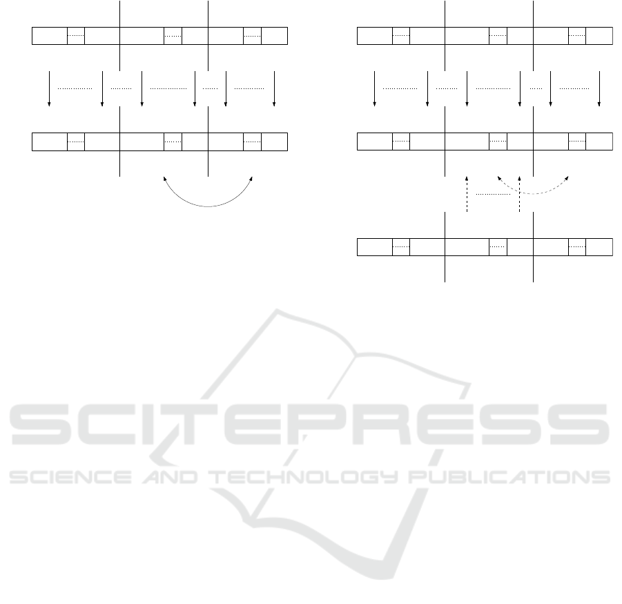
⌈βp⌉–times
x
r
j,1
(s)
x
r
j,(i−1)p
(s)
x
r
j,(i−1)p+1
(s)
x
r
j,ip
(s)
x
r
j,ip+1
(s)
x
r
j,mp
(s)
i-th MUX
Flows already allocated
to (i − 1) MUXes
Remaining (m − i)
x
r
j
(s)
u
j
(s)
all n
elements
u
j,1
(s)
u
j,(i−1)p
(s)
u
j,(i−1)p+1
(s)
u
j,ip
(s)
u
j,ip+1
(s)
u
j,mp
(s)
i-th MUX
Flows already allocated
to (i − 1) MUXes
Remaining (m − i)
copy of
MUXes
MUXes
Figure 2: The mutation operator used to produce a trial vec-
tor u
j
(s) from a random individual x
r
j
(s) selected from cur-
rent population for a parent x
j
(s) for the i-th MUX in itera-
tion s using dβpe swaps.
would have been damaged or completely lost.
Thus, the mutation operator considers only ele-
ments with indices (i − 1)p + 1,... ,mp. It performs
dβpe swaps. In more detail, it randomly selects one
element from the elements with indices (i − 1)p +
1,. . .,ip and one element from elements with indices
ip + 1,. . .,mp in each swap from dβpe swaps and
swaps them. To sum it up, a detailed diagram of the
mutation operator is shown in Figure 2.
β is the scaling factor, controlling the amplifica-
tion of the differential variation. Theoretically β ∈
(0,∞), but it is usually taken from the range [0.1, 1].
3.2 Crossover Operator
The MDE crossover operator implements a discrete
recombination of the trial vector u
j
(s) and the par-
ent vector x
j
(s) to produce offspring x
0
j
(s). x
i, j
(s)
refers to the j-th element of the vector x
i
(s). Elements
u
i, j
(s) and x
0
i, j
(s) are defined in the same way and re-
fer to the j-th element of vectors x
i
(s) and u
i
(s), re-
spectively. CR is the crossover or recombination rate
in the range [0,1].
The approach is similar to the mutation operator.
Let the first (i − 1) MUXes be already allocated. In
general, the crossover operator tries to cross the i-th
MUX only. Firstly, all n elements from the parent
x
j
(s) are copied to the offspring x
0
j
(s). Actually, flows
represented by elements with indices 1, ... , (i − 1)p
have already been allocated to the first (i−1) MUXes.
Therefore, the crossover operator does not consider
elements with indices 1,.. . ,(i − 1)p and leaves them
as they are copied from the parent x
j
(s). By analogy
with the mutation operator, the so far achieved solu-
tion would be damaged or completely lost.
x
j,1
(s)
x
j,(i−1)p
(s)
x
j,(i−1)p+1
(s)
x
j,ip
(s)
x
j,ip+1
(s)
x
j,mp
(s)
i-th MUX
Flows already allocated
to (i − 1) MUXes
Remaining (m − i)
x
j
(s)
x
′
j
(s)
u
j
(s)
all n
elements
if rand(k) ≤ C R k ∈ {(i − 1)p + 1, . . . , ip}
then find element
with value x
′
j,k
(s) in x
′
j
(s)
in x
′
j
(s) with value u
j,k
(s) and swap it
x
′
j,1
(s)
x
′
j,(i−1)p
(s)
x
′
j,(i−1)p+1
(s)
x
′
j,ip
(s)
x
′
j,ip+1
(s)
x
′
j,mp
(s)
i-th MUX
Flows already allocated
to (i − 1) MUXes
u
j,1
(s)
u
j,(i−1)p
(s)
u
j,(i−1)p+1
(s)
u
j,ip
(s)
u
j,ip+1
(s)
u
j,mp
(s)
i-th MUX
Flows already allocated
to (i − 1) MUXes
copy of
x
′
j,l
(s) l ∈ {(i − 1)p + 1, . . . , mp}
MUXes
Remaining (m − i)
MUXes
Remaining (m − i)
MUXes
Figure 3: The crossover operator used to produce an off-
spring x
0
j
(s) from a parent x
j
(s) and a trial vector u
j
(s) for
the i-th MUX in iteration s.
Thus, the crossover operator considers only the el-
ements with indices (i − 1)p + 1,.. .,mp. Then, for
each element
x
0
j,(i−1)p+1
(s),. ..,x
0
j,ip
(s), (9)
if
rand(k) ≤ CR k ∈ {(i − 1)p + 1,. . .,ip}, (10)
then find element
x
0
j,l
(s) l ∈ {(i − 1)p + 1, ... , mp} (11)
in x
0
j
(s) with value u
j,k
(s) and swap the values of ele-
ment x
0
j,k
(s) and element x
0
j,l
(s) in x
0
j
(s). If the condi-
tion in Equation 10 is not satisfied, then do nothing.
In Figure 3, a diagram of the crossover operator
is given. The dashed arrows represent actions being
subjected to the condition in Equation 10. Once the
condition is not satisfied for a given element, it does
nothing and continues to the next element.
3.3 Adaptive Parameters
The scaling factor β and recombination rate CR af-
fect the exploration and exploitation of the algorithm
(Das et al., 2005). Exploration is the algorithm abil-
ity to cover and explore different areas in the feasible
search space while exploitation is the ability to con-
centrate only on promising areas in the search space
and to enhance the quality of the potential solution in
the promising region. The scaling factor β controls
the amplification of the differential variations. The
smaller the value of β, the smaller the mutation step
ECTA 2019 - 11th International Conference on Evolutionary Computation Theory and Applications
216

sizes, and the longer it will take for the algorithm to
converge. Larger values of β facilitate exploration,
but may cause the algorithm to overshoot good op-
tima. The value of β should be small enough to allow
differentials to explore tight valleys, and large enough
to maintain diversity. In this paper, an adaptive scal-
ing factor is adopted to achieve a favorable compro-
mise between exploration and exploitation. For in-
creasing exploration, a large initial value of β is cho-
sen. Then, it is reduced linearly along the iterations
for good exploitation:
β(s) = c
1
− c
2
s
s
max
, (12)
where s
max
is the maximum number of iterations and
c
1
,c
2
are constants. In this way, the mutation operator
performs a wider search in the solution space at the
early stages of the evolution and at the later stages,
the search is restricted around the local area.
The probability of recombination, CR, has a di-
rect influence on a diversity of the MDE. The higher
the probability of recombination, the more variation
is introduced in a new population, thereby increasing
diversity and exploration. Increasing CR often results
in faster convergence, while decreasing CR increases
search robustness. In the MDE, CR is changed along
the evolution process like β as follows:
CR(s) = k
1
− k
2
s
s
max
, (13)
where s
max
is the maximum number of iterations and
k
1
,k
2
are constants.
3.4 Selection Mechanism
In the MDE, a probabilistic selection mechanism (Das
et al., 2007) is used instead of the deterministic selec-
tion of the original DE. The selection mechanism has
been inspired by Simulated Annealing (SA) (Dela-
haye et al., 2019). SA uses a random search strategy,
which not only accepts new solutions that decrease
the objective function value (assuming a minimiza-
tion problem), but may also accept new solutions that
rather increase the objective function value based on
a predetermined probability distribution function. Ex-
ponential probability distribution function is normally
used for this purpose. Based on this idea, the selection
mechanism of the MDE can be described as follows:
x
j
(s + 1) =
x
0
j
(s) if f (x
0
j
(s)) ≤ f (x
j
(s))
x
0
j
(s) if f (x
0
j
(s)) > f (x
j
(s)) ∧
h(x
j
(s),x
0
j
(s)) > rand()
x
j
(s) otherwise,
(14)
h(x
j
(s),x
0
j
(s)) = exp
f (x
j
(s)) − f (x
0
j
(s))
f (x
j
(s))T
!
, (15)
where T is the temperature, as defined in the SA tech-
nique. Here, the temperature T is adaptively changed
in the evolution process as follows:
T (s + 1) = αT (s)
T (0) = T
0
.
(16)
The parameter α is the rate of reducing the tem-
perature (α < 1). T
0
is the initial temperature. A nor-
malized difference between the parent and offspring
objective functions has been considered in Equation
15 to eliminate the effect of different ranges of objec-
tive functions. The selection mechanism begins with
a large value for T
0
and thus, many new worse solu-
tions x
j
(s) have a chance to be selected to increase the
exploration of the MDE. However, the temperature T
decreases along the iterations and so the probability
of selecting worse solutions is decreased.
3.5 The MDE Algorithm
The MDE algorithm consists of the following steps,
the objectives of which are described below:
Step 1 – Parameter Setup
To determine the size of the population N
p
∈ N,
the maximum number of iterations s
max
, constants
c
1
,c
2
,k
1
,k
2
,α and the initial temperature T
0
.
Step 2 – Initialization of Population
To initialize the individuals of the population ran-
domly by the assignment of the input values.
Step 3 – Evaluation of Population
To evaluate the f itness of each individual accord-
ing to the objective function in Equation 1.
Step 4 – Mutation Operation (see Subsection 3.1)
The MDE mutation operator produces a trial vec-
tor u
i
(s) for each individual (parent) x
i
(s) of the
current population. This trial vector will then be
used by the crossover operator to produce off-
spring.
Step 5 – Crossover (see Subsection 3.2)
The MDE crossover operator implements a dis-
crete recombination of the trial vector u
i
(s) and
the parent vector x
i
(s) to produce offspring x
0
i
(s).
Step 6 – Selection (see Subsection 3.4)
Either the parent x
i
(s) or the produced offspring
x
0
i
(s) survives and enters the next generation. To
construct the population of the next generation,
the MDE selection mechanism based on probabil-
ity is used.
Step 7 – Stopping Criterion
If the stopping criterion is not satisfied, go to Step
3, else return the individual with the best f itness
as the solution. Here, the maximum number of
iterations s
max
is selected as the stopping criterion.
Modified Differential Evolution in the Load Balancing Problem for the iFDAQ of the COMPASS Experiment at CERN
217

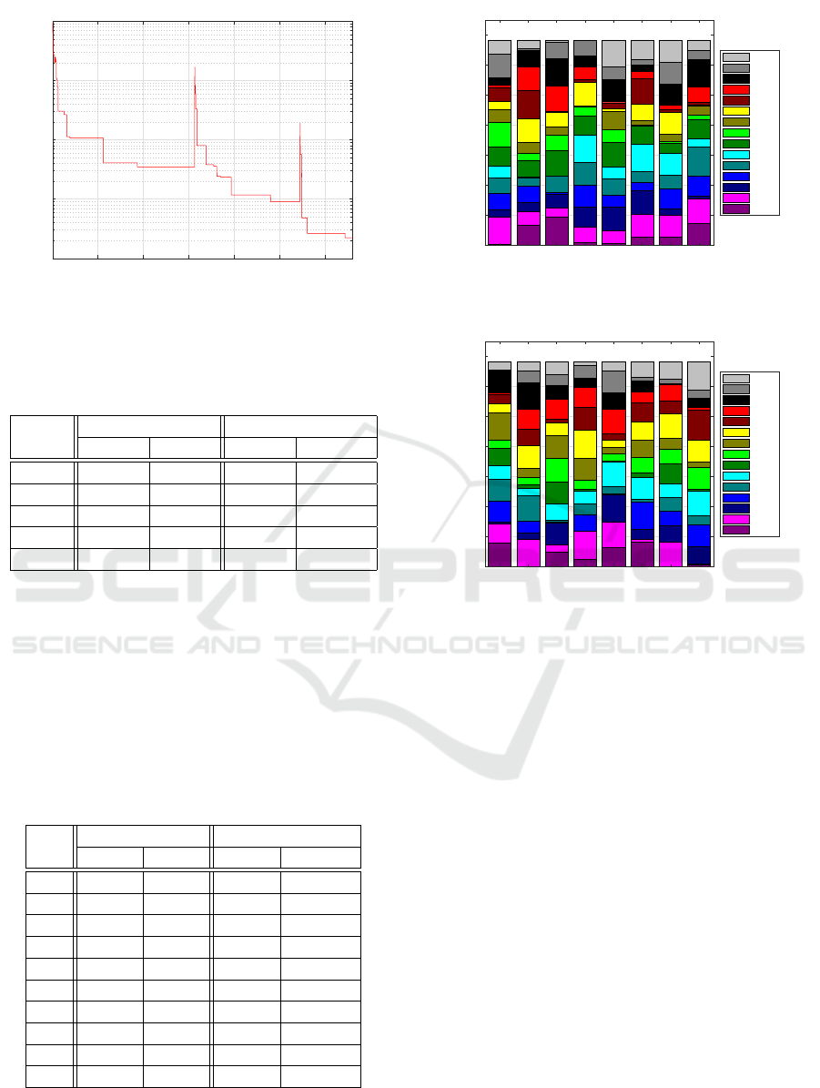
Table 1: Parameters used for the MDE.
N
p
s
max
c
1
c
2
k
1
k
2
T
0
α
50 20,000 0.6 0.4 0.3 0.1 1 0.7
Table 2: The TC1 results using the MDE in each execution.
Ex.
C++ Matlab
Error t [ms] Error t [ms]
1 2.24 1,601 2.24 71,413
2 2.24 1,652 2.24 25,558
3 2.24 1,997 2.24 23,688
4 2.24 2,220 2.24 25,378
5 2.24 1,382 2.24 43,370
6 2.24 2,099 2.24 90,298
7 2.24 862 2.24 78,666
8 2.24 1,901 2.24 71,448
9 2.24 2,379 2.24 57,260
10 2.24 1,803 2.24 28,210
4 NUMERICAL RESULTS
The MDE has been implemented in C++ and Mat-
lab (R2018a, 64-bit) on a personal computer equipped
with Intel(R) Core(TM) i7-8750H CPU (@2.20 GHz,
6 Cores, 12 Threads, 9M Cache, Turbo Boost up to
4.10 GHz) and 16 GB RAM (DDR4, 2 666 MHz)
memory. The MDE is examined on two test cases and
numerical results are compared with other methods of
solving the LB problem.
The results are investigated with respect to the er-
ror and computation time. The error is defined as the
objective function of the LB problem, see Equation 1.
4.1 Test Case 1
The Test Case 1 (TC1) consists of m = 6 MUXes with
p = 15 ingoing ports each and with respect to the
number of MUXes, it corresponds to the iFDAQ setup
used in the COMPASS Run 2016, 2017 and 2018. It
considers n = m · p = 6 · 15 = 90 flows with values
randomly generated in the range from 0 B to 10 kB.
The proposed MDE algorithm is partially stochas-
tic and hence, it might produce different solutions in
every execution. The parameters used for the MDE
algorithm to solve the TC1 are given in Table 1.
In Table 2, the results produced in C++ and Mat-
lab for the TC1 using the MDE in each execution
are stated. The error is equal approximately to 2.24
giving a global optimum in each execution, however,
the solutions might be different – multiple global op-
tima are possible. The best TC1 flow allocation based
on the MDE produced in C++ corresponding to Ex-
82,494
82,493 82,493 82,493 82,493 82,493
MUX
1
MUX
2
MUX
3
MUX
4
MUX
5
MUX
6
0
10,000
20,000
30,000
40,000
50,000
60,000
70,000
80,000
90,000
Flow [B]
Port 15
Port 14
Port 13
Port 12
Port 11
Port 10
Port 9
Port 8
Port 7
Port 6
Port 5
Port 4
Port 3
Port 2
Port 1
Figure 4: The best TC1 flow allocation based on the MDE
produced in C++ corresponding to Execution 7.
82,494
82,493 82,493 82,493 82,493 82,493
MUX
1
MUX
2
MUX
3
MUX
4
MUX
5
MUX
6
0
10,000
20,000
30,000
40,000
50,000
60,000
70,000
80,000
90,000
Flow [B]
Port 15
Port 14
Port 13
Port 12
Port 11
Port 10
Port 9
Port 8
Port 7
Port 6
Port 5
Port 4
Port 3
Port 2
Port 1
Figure 5: The best TC1 flow allocation based on the MDE
produced in Matlab corresponding to Execution 3.
ecution 7 is given in Figure 4 and produced in Mat-
lab corresponding to Execution 3 is given in Figure
5. In both figures, the total flow allocated to the first
MUX is 82,494 B and to the remaining five MUXes is
82,493 B each. Thus, the mutual comparison reaches
82,493/82, 494 ≈ 100.00%. The computational time
is very low in C++ due to the fast memory access pro-
vided by C++ and the usage of pointers trying to avoid
any copying of memory. Hence, the MDE algorithm
represents a good candidate for a real-time LB solver.
To demonstrate the behaviour of the MDE algo-
rithm, the evolution process of the best TC1 flow al-
location produced in Matlab corresponding to Execu-
tion 3 is shown in Figure 6. At the beginning of the
evolution process, it shows a fast convergence of the
proposed MDE algorithm. It reached a solution close
to a global optimum after just 150 iterations. Never-
theless, there are several short-term deteriorations of
the error in evolution, which are caused by selection
mechanism based on SA. The selection mechanism
sometimes selects individuals with a worse f itness
value. They have a chance to show their potential
to produce a new population. However, this feature
weakens at the end of the evolution process.
ECTA 2019 - 11th International Conference on Evolutionary Computation Theory and Applications
218
0 500 1,000 1,500 2,000 2,500 3,000
Iteration
10
0
10
1
10
2
10
3
10
4
Error
Figure 6: The evolution process of the best TC1 flow alloca-
tion based on the MDE produced in Matlab corresponding
to Execution 3.
Table 3: Comparison of LB solution methods based on the
best flow allocation for the TC1.
Met.
C++ Matlab
Error t [ms] Error t [ms]
DP 2.24 17,529 2.24 16,521
GH 243.89 47 243.89 1
ILP 21.19 17,127 23.81 1,465
MDE 2.24 862 2.24 23,688
RL 10.44 32,404 10.44 117,106
Finally, a global optimum is reached after 3,400
iterations and the error is equal approximately to 2.24.
The TC1 results produced by the MDE are com-
pared with other LB solution methods – Dynamic
Programming (DP), Greedy Heuristic (GH), Integer
Linear Programming (ILP) and Reinforcement Learn-
ing (RL) – in Table 3. In sum, the MDE and GH, both
reaching a global optimum, can be used for real-time
LB due to the low computational time.
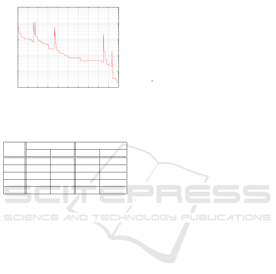
Table 4: The TC2 results using the MDE in each execution.
Ex.
C++ Matlab
Error t [ms] Error t [ms]
1 15.30 6,050 2.00 87,064
2 2.00 2,507 2.00 67,601
3 2.00 1,911 2.00 104,993
4 2.00 3,266 2.00 61,987
5 2.00 2,358 2.00 94,706
6 2.00 2,659 2.00 80,280
7 2.00 5,398 4.24 151,224
8 2.00 3,153 2.00 108,325
9 2.00 2,718 2.00 37,530
10 2.00 5,100 2.00 82,067
68,401 68,401 68,401 68,401
68,400 68,400 68,400 68,400
MUX
1
MUX
2
MUX
3
MUX
4
MUX
5
MUX
6
MUX
7
MUX
8
0
10,000
20,000
30,000
40,000
50,000
60,000
70,000
Flow [B]
Port 15
Port 14
Port 13
Port 12
Port 11
Port 10
Port 9
Port 8
Port 7
Port 6
Port 5
Port 4
Port 3
Port 2
Port 1
Figure 7: The best TC2 flow allocation based on the MDE
produced in C++ corresponding to Execution 3.
68,401 68,401 68,401 68,401
68,400 68,400 68,400 68,400
MUX
1
MUX
2
MUX
3
MUX
4
MUX
5
MUX
6
MUX
7
MUX
8
0
10,000
20,000
30,000
40,000
50,000
60,000
70,000
Flow [B]
Port 15
Port 14
Port 13
Port 12
Port 11
Port 10
Port 9
Port 8
Port 7
Port 6
Port 5
Port 4
Port 3
Port 2
Port 1
Figure 8: The best TC2 flow allocation based on the MDE
produced in Matlab corresponding to Execution 9.
4.2 Test Case 2
The Test Case 2 (TC2) consists of m = 8 MUXes with
p = 15 ingoing ports each and thus, it corresponds
to the iFDAQ full setup. However, the iFDAQ full
setup has never been in operation for the COMPASS
experiment since it was not required by any physics
program. It considers n = m · p = 8 · 15 = 120 flows
with values randomly generated in the range from 0 B
to 10 kB. The parameters used for the MDE algorithm
to solve the TC2 are the same as for TC1, see Table 1.
In Table 4, the results produced in C++ and Mat-
lab for the TC2 using the MDE in each execution
are stated. The error is almost always equal to 2.00
giving a global optimum in each execution. The
best TC2 flow allocation based on the MDE pro-
duced in C++ corresponding to Execution 3 is given
in Figure 7 and produced in Matlab corresponding to
Execution 9 is given in Figure 8. In both figures,
the total flow allocated to the first four MUXes is
68,401 B each and to the remaining four MUXes is
68,400 B each. Thus, the mutual comparison reaches
68,400/68, 401 ≈ 100.00%.
Modified Differential Evolution in the Load Balancing Problem for the iFDAQ of the COMPASS Experiment at CERN
219
0 500 1,000 1,500 2,000 2,500 3,000 3,500 4,000 4,500 5,000
Iteration
10
0
10
1
10
2
10
3
10
4
10
5
Error
Figure 9: The evolution process of the best TC2 flow alloca-
tion based on the MDE produced in Matlab corresponding
to Execution 9.
Table 5: Comparison of LB solution methods based on the
best flow allocation for the TC2.
Met.
C++ Matlab
Error t [ms] Error t [ms]
DP 2.00 24,873 2.00 23,873
GH 224.22 63 224.22 1
ILP 194.43 49,927 134.61 95,251
MDE 2.00 1,911 2.00 37,530
RL 2.83 75,882 2.45 204,824
The evolution process of the best TC2 flow allo-
cation based on the MDE produced in Matlab corre-
sponding to Execution 9 can be seen in Figure 9. A
global optimum is reached after 4,900 iterations and
the error is equal to 2.00. Finally, the TC2 results
produced by the MDE are compared with results ac-
quired by DP, GH, ILP and RL in Table 5.
5 CONCLUSION
The paper has introduced the LB problem of the iF-
DAQ of the COMPASS experiment at CERN. N P -
completeness of the LB problem makes optimiza-
tion more challenging. The proposed MDE has a
new crossover and mutation operator and its selection
mechanism is inspired by SA. Results have shown the
MDE matches requirements in terms of the best error
and ability to find a global optimum. Thus, the MDE
represents a solver of the long-term LB setup, where
no frequent changes in the flows are expected.
Since 2019, a crosspoint switch connecting all
involved links in the iFDAQ provides a fully pro-
grammable system topology making the iFDAQ re-
configurable on-the-fly and replaces the fixed point-
to-point connections. Thus, the crosspoint switch will
analyze flows and automatically assign them to input
ports of MUXes in order to equally distribute load
over all MUXes. The low computational time of the
MDE opens up a perspective for real-time LB.
ACKNOWLEDGEMENTS
This research has been supported by OP VVV, Re-
search Center for Informatics, CZ.02.1.01/0.0/0.0/
16 019/0000765.
REFERENCES
Affenzeller, M., Wagner, S., Winkler, S., and Beham, A.
(2018). Genetic Algorithms and Genetic Program-
ming: Modern Concepts and Practical Applications.
Taylor & Francis Ltd, first edition.
Alexakhin, V. Y. et al. (2010). COMPASS-II Proposal. The
COMPASS Collaboration. CERN-SPSC-2010-014,
SPSC-P-340.
Bodlak, M. et al. (2014). FPGA based data acquisition sys-
tem for COMPASS experiment. Journal of Physics:
Conference Series, 513(1):012029.
Bodlak, M. et al. (2016). Development of new data ac-
quisition system for COMPASS experiment. Nuclear
and Particle Physics Proceedings, 273(Supplement
C):976–981. 37th International Conference on High
Energy Physics (ICHEP).
Das, S., Konar, A., and Chakraborty, U. K. (2005). Two
Improved Differential Evolution Schemes for Faster
Global Search. In GECCO 2005 – Genetic and Evo-
lutionary Computation Conference, pages 991–998.
Das, S., Konar, A., and Chakraborty, U. K. (2007). An-
nealed Differential Evolution. In 2007 IEEE Congress
on Evolutionary Computation, pages 1926–1933.
Das, S., Mullick, S. S., and Suganthan, P. N. (2016). Re-
cent Advances in Differential Evolution -– An Up-
dated Survey. Swarm and Evolutionary Computation,
27:1–30.
Delahaye, D., Chaimatanan, S., and Mongeau, M. (2019).
Simulated Annealing: From Basics to Applications,
pages 1–35. Springer International Publishing.
Eiben, A. E. and Smith, J. E. (2015). Introduction to Evo-
lutionary Computing. Springer-Verlag Berlin Heidel-
berg, second edition.
Kameda, H., Li, J., Kim, C., and Zhang, Y. (1997). Op-
timal Load Balancing in Distributed Computer Sys-
tems. Springer-Verlag London, first edition.
Kellerer, H., Pferschy, U., and Pisinger, D. (2004). Knap-
sack Problems. Springer-Verlag Berlin Heidelberg,
Berlin, Germany, first edition. ISBN 978-3-540-
24777-7.
Storn, R. and Price, K. (1995). Differential Evolution:
A Simple and Efficient Adaptive Scheme for Global
Optimization Over Continuous Spaces. Journal of
Global Optimization, 23.
ECTA 2019 - 11th International Conference on Evolutionary Computation Theory and Applications
220
