Deep Semantic Feature Detection from Multispectral Satellite Images

Hanen Balti

, Nedra Mellouli

, Imen Chebbi

, Imed Riadh Farah

and Myriam Lamolle

RIADI Laboratory, University of Manouba, Manouba, Tunisia

LIASD Laboratory, University of Paris 8, Paris, France

Keywords:

Big Data, Remote Sensing, Feature Detection, CNN, Semantic Segmentation.

Abstract:

Recent progress in satellite technology has resulted in explosive growth in volume and quality of high-

resolution remote sensing images. To solve the issues of retrieving high-resolution remote sensing (RS) data

in both efﬁciency and precision, this paper proposes a distributed system architecture for object detection in

satellite images using a fully connected neural network. On the one hand, to address the issue of higher com-

putational complexity and storage ability, the Hadoop framework is used to handle satellite image data using

parallel architecture. On the other hand, deep semantic features are extracted using Convolutional Neural

Network (CNN),in order to identify objects and accurately locate them. Experiments are held out on several

datasets to analyze the efﬁciency of the suggested distributed system. Experimental results indicate that our

system architecture is simple and sustainable, both efﬁciency and precision can satisfy realistic requirements.

1 INTRODUCTION

Earth Observation (EO) is an approach of collecting

data about planet Earth through satellite imaging. The

location where we can obtain most of our planet’s data

is in orbit. Remote sensing (RS) satellite data pro-

cessing is one of the complicated tasks of image pro-

cessing since big, sophisticated data are processed.

It ﬁnds a huge of applications in ﬁelds such as me-

teorology, geology, forestry, seismology, oceanogra-

phy, etc. Datasets may contain images of distinct

sensors, distinct viewing angles and distinct viewing

times. Satellite images have distinctive issues such

as cloud pixels, noise in images, systemic mistakes,

multi-spectral images, distortions of terrain, etc.To

manage satellite imagery preprocessing, we need to

use an elaborate computational structure such as the

Hadoop Framework.

Hadoop is an open source distributed frame-

work based on the processing technique of Google

MapReduce and the distributed structure of the

ﬁle system. The Hadoop framework is composed

of principally of Hadoop Distributed File System

(HDFS) (D.Borthakur, 2018a) and Hadoop MapRe-

duce (D.Borthakur, 2018b). HDFS is a distributed

ﬁle system that holds big amounts of data and offers

strong access to information throughput. HDFS is ex-

tremely tolerant to faults and is intended for low-cost

hardware deployment. Data is divided into smaller

parts in the Hadoop cluster and spread across the clus-

ter. HDFS primary objective is to reliably store data

even in presence of errors including name node fail-

ure, data node failure, and network partition failures.

MapReduce is a programming model intended to pro-

cess huge volumes of data in parallel by separating

job into individual tasks. MapReduce main objective

is to divide input information set into separate parts

that are processed in a fully parallel way. For the data

stored in Hadoop Framework retrieval, there are many

methods and technologies such as Handcrafted meth-

ods, Machine learning and so on; in our work, we will

be concentrated on Deep Learning.

Deep learning (DL) is a machine learning sub-

group, referring to the implementation and variations

of a collection of algorithms called neural networks.

With these methods, you can use the network to learn

or train on a number of labeled samples (Wang et al.,

2016). The labeling of these samples is performed in

many ways. Machine learning feature extraction is

performed manually and classiﬁcation is performed

by the machine. However, both the extraction of the

feature and the classiﬁcation are performed by ma-

chine in deep learning. The Deep Learning neural

network is therefore more efﬁcient in identifying the

Satellite Imagery. In addition, semantic information

gathered from deep neural networks can be used for

image retrieval to improve search efﬁciency.

Remote sensing data volume and heterogeneity

458

Balti, H., Mellouli, N., Chebbi, I., Farah, I. and Lamolle, M.

Deep Semantic Feature Detection from Multispectral Satellite Images.

DOI: 10.5220/0008350004580466

In Proceedings of the 11th International Joint Conference on Knowledge Discovery, Knowledge Engineering and Knowledge Management (IC3K 2019), pages 458-466

ISBN: 978-989-758-382-7

are considered as two separate challenging issues in

the litterature. Our research aims to suggest an adap-

tive structure to address the issue of scaling up and

processing large volume of remote sensing data using

Hadoop Framework and DL. In this work, we pro-

pose an approach that uses DL architecture for data

processing and Hadoop HDFS for data storage. Sec-

tion 2 offers a short survey of some related works.

Section 3 describes the proposed approach for remote

sensing data processing. In Section 4, we describe

data source, software and hardware conﬁguration and

results obtained. Section 5 concludes the paper.

2 RELATED WORKS

The amount and quality of satellite images have been

greatly improved with the growth of satellite technol-

ogy. These data can not be processed using stan-

dard techniques. Although parallel computing and

cloud infrastructure (Hadoop, Spark, Hive, HBase,

etc.) make it possible to process such massive data,

such systems are sufﬁcient for spatial and temporal

data.

Some works were performed on raster images

in the literature using MapReduce programming

paradigm. (Cary et al., 2009) presented MapRe-

duce model for the resolution of two major vec-

tor and raster data spatial issues: R-Trees bulk con-

struction and aerial image quality computation. Im-

agery data is stored in a compressed DOQQ (A Dig-

ital Orthophoto Quadrangle and Quarter Quadrangle)

ﬁle format, and Mapper and Reducer process those

ﬁles. (Golpayegani and Halem, 2009) implements

some image processing algorithms using MapReduce

model. Indeed, the ﬁrst step is to convert images to

text format and then to binary format before using

them as a raw image. In contrast, (Almeer, 2012) pre-

sented a six-fold speedup for auto-contrast and eight-

fold speedup for the sharpening algorithm. (Kocaku-

lak and Temizel, 2011) used Hadoop and MapReduce

to operate a ballistic image analysis that needs a volu-

minous image database to be paired with an unknown

image. It was shown that the processing time was

lowered dramatically as 14 computational nodes were

in cluster setup. This method used a high computa-

tional requirement. (Li et al., 2010) tried to decrease

the time required for computing the huge amount of

satellite images using Hadoop and MapReduce meth-

ods for running parallel clustering algorithms. The

method begins with the clustering of each pixel and

then computes all current cluster centers according to

each pixel in a collection of clusters. (Lv et al., 2010)

suggested a different clustering algorithm that uses a

K-means strategy to remote sensing image process-

ing. Objects with matching spectral values, without

any formal knowledge, are grouped together. The

Hadoop MapReduce strategy supported the parallel

K-means strategy, as the algorithm is intensive both

in time and in memory. All these works concentrate

essentially on parallel processing using the Hadoop

Map-Reduce framework for image data.

For the remote sensing data processing task using

DL, Convolutional Neural Network (CNN) has shown

important enhancement in image similarity task as-

signments as the latest effective deep learning branch.

The concept that deep convolutional networks can re-

trieve high-level features in the deeper layers led by

the researchers to investigate methods this technique

can decrease the semantic gap.The extracted features

can be used as image representations in search algo-

rithms on both fully connected layers and convolution

layers. (Sun et al., 2016) proposed a method based on

CNN that extract features from local regions, in ad-

dition of extracting features from the whole images.

(Gordo et al., 2017) merged RMAC (Regional Max-

imal ACtivation) with triplet networks and also sug-

gested a regional proposal network (RPN) strategy for

the identiﬁcation of the region of interest (RoI) and

the extraction of local RMAC descriptors. (Zhang

et al., 2015) proposed a gradient boosting random

convolutional network (GBRCN) to rank very high

resolution (VHR) satellite imagery. A sum of func-

tions (called boosts) are optimized in GBRCN. For

optimization, a modiﬁed multi-class softmax func-

tion is used, making the optimization job simpler,

SGD is used for optimization. (Zhong et al., 2017)

used reliable tiny CNN kernels and profound archi-

tecture to learn about hierarchical spatial relationships

in satellite data. An output class label of a softmax

classiﬁer based on CNN DL inputs. The CPU han-

dles preprocessing (data splitting and normalization),

while the GPU runs convolution, ReLU and pooling

tasks, and the CPU handles dropout and softmax clas-

siﬁcation. Networks with one to three convolution

layers are evaluated, with receptive ﬁelds. In order

to estimate region boundary conﬁdence maps which

are then interfused to create an aggregate conﬁdence

map, (Basaeed et al., 2016) used a CNN committee

that conducts a multi-size analysis for each group.

(Längkvist et al., 2016) used the CNN in multispec-

tral images (MSI) for a complete, quick and precise

pixel classiﬁcation, with a small cities digital surface

design. In order to improve the high level segmen-

tation, the low level pixel classes are then predicted.

The CNN architecture is evaluated and is analyzed.

(Marmanis et al., 2016) have tackled the prevalent

RS issue of restricted training information by using

Deep Semantic Feature Detection from Multispectral Satellite Images

459

domain-speciﬁc transfer learning. They used the Im-

ageNet dataset with a pre-trained CNN and extracted

the ﬁrst set of orthoimagery depictions. These repre-

sentations are then transmitted to a CNN classiﬁca-

tion. A novel cross-domain fusion scheme was cre-

ated in this study. Their architecture has seven con-

volutional layers, two long Multi Perceptron (MLP)

layers, three convolutional layers, two larger MLP

layers, and a softmax classiﬁer. The features are ex-

tracted from the last layer. (Donahue et al., 2014) re-

search has shown that deeper layers contain the ma-

jority of the discriminatory information. Moreover,

they are equipped with features from the large (1 x 1 x

4096) MLP, a very long output of the vector and con-

vert it into 2D feature array with a large mask layer

(91 x 91), this is achieved because the large feature

vector is a computational bottleneck, while the 2D

data can be processed very efﬁciently via a second

CNN. This strategy works if the second CNN is able

to understand data through its layers in the 2D rep-

resentation. This is a very distinctive strategy which

raises some interesting questions concerning alterna-

tive DL architectures, this strategy was also success-

ful, since the characteristics of the initial CNN in the

new image domain were efﬁcient.

The heterogeneity of input images as well as their

scaling are regarded independently in all the works

mentioned above. Our research aims to handle an

adaptive structure framework to address the issue of

scaling up and processing large volume of remote

sensing data combining Hadoop and DL systems.

3 PROPOSED APPROACH

Big remote sensing data processing is challenging.

The volume and heterogeneity actually presents is-

sues for this kind of data processing, and that is why,

to resolve this issue, we suggest a distributed archi-

tecture with DL model for data processing (Figure 1).

Our approach consists of 4 steps: (1) image storing;

(2) data processing and labelling; (3) data fusion .

3.1 Image Storing

A multi-spectral image is a compilation of various

monochrome images taken with a distinct sensor from

the same aerial scenes. Each image is termed a band.

Multi-spectral images are most frequently used for re-

mote sensing applications in image processing. Satel-

lites generally take several images in the visual and

non-visual spectrum from frequency bands.

There are many techniques for image processing

where we can do image processing. But the principal

drawback is that this machine-optimized tools are in

nature sequential. It would be a long time to process

large amounts of high-resolution remote sensing im-

ages when processing Remote Sensing Data (image

by image). That is why in our work, we will treat ev-

ery band separetly in a parallel way. We, therefore,

need a multi-speciﬁc framework that can apply par-

allelism in the most efﬁcient way and guarantee that

every data is processed safely. Hadoop supplies this.

Besides, in moving the computation towards the pro-

cessing node instead of moving the data the princi-

ple of Hadoop implementation, ensures data-location.

The volume of output data is much larger than the

computation involved when handling high-resolution

remote sensing satellite images. Based on this, it can

be concluded that the Hadoop framework suits this

task best.

As a preprocessing step, before running the appli-

cation, we must save the remote sensing image ﬁles in

HDFS. This step is devided in three sub-steps (Figure

2).

First, we must split the image «Band»(B) in m

parts. The input image is chosen from the local ﬁle

system input folder, I

input

. For each input image,

B performs split operation if the image dimension

is greater than the predeﬁned dimension. Generated

split band ﬁles (segments) (S

to S

) are placed in

the directory that is produced with the name of the

ﬁle as the image name. Secondly, a serialization step

of strips of bands is achieved. In this phase, each

group of split band ﬁles is transformed into a seri-

alized structure. Each folder that contains split im-

ages is selected and its data content is communally

written to a given metadata folder using serialization.

The metadata contain information about the number

of band strips, the ﬁlename, path/row of the band and

the band captured time. The third step is the serializa-

tion for HDFS block. As we have, from the previous

step, a ﬁle that contains the data content and the meta-

data we can now store it in HDFS and do the process-

ing task. Finally, upon completion of the above phase,

all operations during the implementation of MapRe-

duce will use these ﬁles as entries.

3.2 Data Processing

Once we have all our data splitted and stored in HDFS

we are going to perfom the processing step. Firstly,

we will assign each split to a map job.

This is a pseudo-code explaining the job of the

Mapper class:

Class: Mapper

Function: Map

Map(Key(Filename),BytesWritableValue

(SerializedBand<BFi>,Output)

KDIR 2019 - 11th International Conference on Knowledge Discovery and Information Retrieval

460

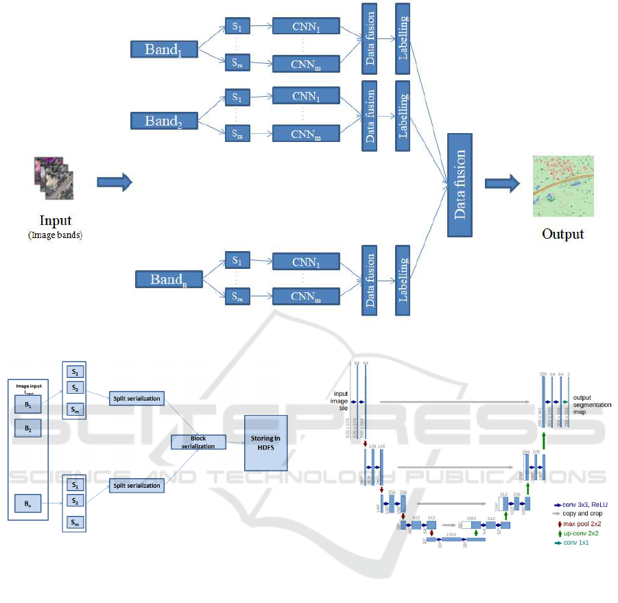
Figure 1: The architecture of the proposed approach.

Figure 2: Preprocessing step.

Foreach BandSplit<Sm>in BFi

Processing(Sm);

SerializedEachMapOutput(OS1..OSm)->OFBi;

Output:

SetKey:Filename==KeyInputToMap;

SetValue:SerializedMapOutput<OFBi>;

In the Mapper, we will treat our strips of images

using UNET which belongs to CNN architecture.

This model makes the shape of the letter «U »that’s

why he is called UNET. It is composed from two

parts: an encoder and a decoder (Figure 3).

UNET was developed by (Ronneberger et al.,

2015) for the segmentation of Bio Medical images.

The architecture contains two paths:

• The ﬁrst path is the contraction path (also called

encoder) used to capture the features in the image.

The encoder is just a traditional stack of convolu-

Figure 3: UNET architecture.

tion and Max Pooling layers.

• The second path is the expansion path (also

known as a decoder) that allows us to locate

objects precisely using transposed convolutions.

Thus, it is a fully end-to-end convolutional net-

work (FCN), without a dense layer for which rea-

son it can accept images of any size.

The encoder consists of 4 blocks. Each block is com-

posed of: two 3x3 convolution layer with activation

function (with batch normalization) and a 2x2 Max

Pooling and the decoder part is symmetrical with the

encoder part, this part consists of transposed convolu-

tion layers and convolutional layers. The processing

is applied on each strip r times in order to detect r

object. In the training step, we added the reﬂectance

indices in order to detect the water or the vegetation

these are some indices. These indices show that fea-

Deep Semantic Feature Detection from Multispectral Satellite Images

461

ture learning is well-related to certain categories of

objects found in the traditional Geographic Informa-

tion System (GIS).

• NDWI(Normalized Difference Water Index):

NDW I =

GREEN − NIR

GREEN + NIR

(1)

• CCCI (Canopy Chlorophyl Content Index):

CCCI =

NIR − REDedge

NIR + REDedge

∗

NIR + RED

NIR − RED

(2)

• EVI (Enhanced Vegetation Index):

EV I = G∗

NIR − RED

NIR +C1 ∗ RED − C2 ∗ BLUE +L

(3)

• SAVI (Soil-Adjusted Vegetation Index):

SAVI =

(1 + L)(NIR − RED)

NIR + RED + L

(4)

where:

- L is an adjustment factor of the canopy back-

ground. L is a constant equal to 0.5;

- G gain factor;

- C1, C2 are the coefﬁcients of the aerosol resis-

tance term, which use the blue band to correct

aerosol inﬂuences in the red band.

Obviously, the idea that we have infrared and other

non-visible frequency range stations permit us to eas-

ily deﬁne certain classes from the pixel values, with-

out any background information. Finally, we obtain a

segmentation map containing the features of each ob-

ject separately in form of a .csv ﬁle (i.e each object is

associated to a csv ﬁle). We merge all these ﬁles in a

single ﬁle. This ﬁle contains the features of the strip.

Once, we obtained several outputs representing

the feature maps of each band they are serialized in

the mapper as mentioned in the Mapper pseudo-code.

The outputs of the mapper job will be assigned to the

Reducer function (Figure 4).

Figure 4: Map job description.

Therefore, the reducer will deserialize the map

outputs and combine the splits.

Class:Reducer

Function: Reduce

Reduce(Key(Filename),BytesWritableValue

(SerializedMapOutput<OFBi>,Output)

Deseiralize_value(OFBi);

Foreach processedBandSplit<OSm> in OBFi

ImageProcessing(Sm);

CombineEachOutput(FS1..FSm)->OBn

SaveReduceOutput(OBn);

Output:

SetKey:Filename==BandFileName;

SetValue:ReduceOutput<OBn>;

For the labelling task, according to its features,

each object will be assigned to a color and a numerical

id.

3.3 Data Fusion and Labelling

At this step, we have the band reconstructed we need

to merge all the bands. The fusion of the bands at-

tempts at thin borders, connecting them to closed con-

tours, and generating a map of hierarchical segmenta-

tion.

For the bands fusion, we used the Wavelet Trans-

form (WT) (Rani and Sharma, 2013). In fact, WT

plays major role in Multi-resolution Analysis in pro-

ducing a representation between spatial and Fourier

domains. Based on their local frequency content, each

image could be measured by decomposing the initial

image into various channels, where decomposition is

provided by discrete two-dimensional WT. There are

ﬁve steps that should by performed in order to perfom

this step.

Firstly, effect upscaling and generate the Inten-

sity (I) image from the upscaled multispectral im-

age, perform the corresponding histogram between

the bands and I image, decompose the bands re-

lated to the Wavelet planes, and ﬁnally apply inverse

Wavelet Transform to get merged multispectral band.

All this work will be performed in the master node.

4 EXPERIMENTS AND RESULTS

In this section, we discuss the experimental setup and

data set used for testing the proposed approach.

4.1 Environmental Setup

Our experiments was performed on 16-node cluster.

In Table 1, we describe the hardware conﬁguration of

the nodes.

4.2 Data Description

The framework that has been created can generally be

used to handle multispectral satellite images. Mul-

tispectral images usually relate to 3 to 10 channels

KDIR 2019 - 11th International Conference on Knowledge Discovery and Information Retrieval

462

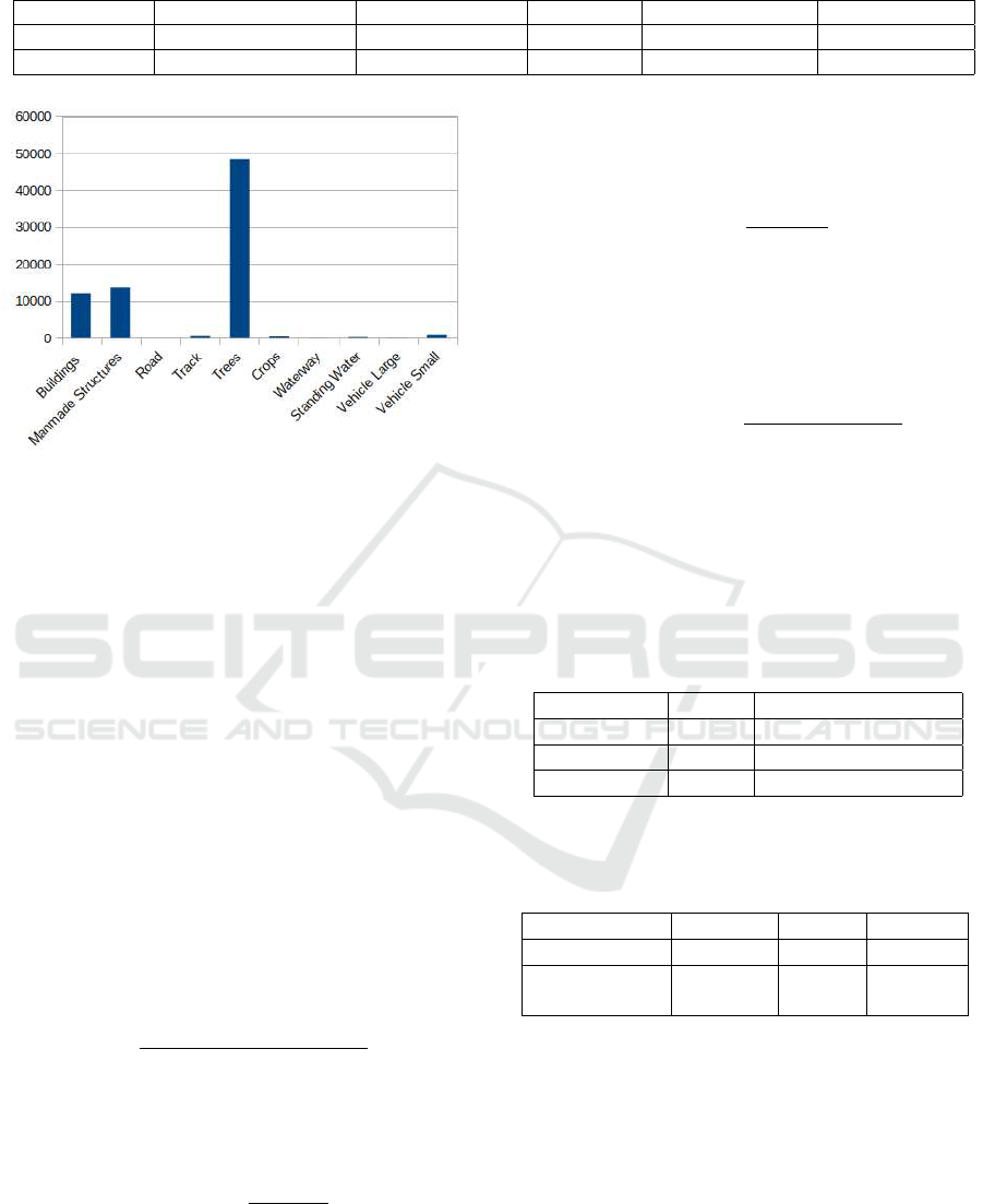
Table 1: Nodes hardware description.

Node Type Memory size (RAM) CPU CPU cores Operating System Hadoop version

Master Node 6 Gbytes Intel i7 3.90 GHz 4 Ubuntu 16.04 2.7

All the Slaves 8 Gbytes Intel i7 3.90 GHz 4 Ubuntu 16.04 2.7

Figure 5: Distribution of labels on the multispectral dataset.

represented in pixels. Using a remote sensing captor,

each band is obtained. The ﬁrst dataset is ISPRS Vai-

hingen (ISPRS, 2019) data which containe 33 RGB

(Red-Green-Blue) images with their ground truth and

several resolutions.

The second dataset contains 450 satellite images

which include both 3-band images (RGB colors)

and 16-bands which are taken from the multispec-

tral (400-1040nm) and short-wave infrared (SWIR)

(1195-2365nm) range with different spatial resolu-

tions.

These images are captured by the commercial sen-

sor WorldView-3 (Corporation, 2017). Figure 5 rep-

resents labels distribution on the multispectral dataset.

4.3 Evaluation Metrics

The ﬁrst metric that we used is the time, then in order

to evaluate the Speedup (S) of our architecture com-

paring to a single node architecture we compute:

S =

SpeedO f aSingleNode

SpeedO f OurArchitecture

(5)

The second metric is the precision: it is the relation of

the number of right predictions to the total number of

input samples.

precision =

T P

T P + FP

(6)

where TP (True Positives) indicates the number of

properly identiﬁed items, FN (False Negatives) the

number of undetected items and FP (False positives)

the amount of wrongly identiﬁed items.

The third metric is the recall: It is the percentage

of the number of predictions relevant to the total num-

ber of samples entered.

recall =

T P

T P + FN

(7)

The fourth metric is the F1-score: F1-Score is the

mean between accuracy and recall. The F1-Score

range is [ 0, 1 ]. It informs you how accurate your

classiﬁer is (how many objects it properly classiﬁes)

and how robust it is.

F1 − score = 2 ∗

Precision ∗ recall

precision + recall

(8)

4.4 Results

In this section, we present the results of our appraoch,

in terms of speed and in term of precision and recall.

Table 2, describes the execution time in minutes

(min) of the proposed architecture compared to a sin-

gle node architecture with the Speedup ratio.

Table 2: Execution times.

Dataset ISPRS Multispectral dataset

Single Node 6.4min 35.2min

MultiNode 1.5min 5.3min

Speedup 4.2 6.71

Table 3 corresponds to the results of the proposed

architecture in term of precision and recall.

Table 3: Results obtained for the two datasets.

Dataset Precision Recall F1-score

ISPRS 90.2 % 81.2 % 85.46%

Multispectral

dataset

94.3% 92.2% 93.24%

Table 4 contains the results that we obtained for

each class in the ISPRS dataset.

Table 5 includes the results obtained for the mul-

tispectral dataset with each class.

Some images are shown to illustrate our results.

Figure 6 represents the 3-band image results where

image (a) is the real RGB image, (b) is the result of

our work. We denote that the objects detected in this

type of image are Imprevious Surfaces, low vegeta-

tion, Buildings, Cars, Trees and Clutter.

For the classiﬁcation of this image we got good

results mentionned in Table 6 .

Deep Semantic Feature Detection from Multispectral Satellite Images

463

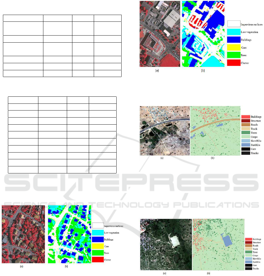
Table 4: Results obtained for each class from the ISPRS

dataset.

Class Precision Recall F1-score

Impervious

surfaces

0.92 0.93 0.92

Building 0.95 0.96 0.95

Low vegeta-

tion

0.84 0.84 0.84

Tree 0.90 0.90 0.90

Car 0.83 0.82 0.82

Clutter 0.97 0.41 0.57

Table 5: Results obtained for each class of the multispectral

dataset.

Class Precision Recall F1-score

Buildings 0.88 0.87 0.87

Cars 0.70 0.64 0.67

Crops 0.83 0.83 0.83

FastH2O 0.38 0.36 0.37

Roads 0.36 0.20 0.26

SlowH2O 0.76 0.62 0.68

Structure 0.95 0.96 0.95

Tracks 0.96 0.95 0.95

Trees 0.98 0.95 0.96

Trucks 0.93 0.94 0.93

As we can notice in Figure 6 and in Table 6, there

is no clutter detected as there is no clutter in the orig-

inal RGB image.

Figure 6: RGB images results (a) is the RGB image, (b) is

the result of our work.

Figure 7 is another RGB classiﬁcation, in which

we had some results not good as the ﬁrst image, here

Table 7 in which we present the results. For example,

clutter detection had the accuracy of 98%, recall 60%

and F1-score 75%. This can be explained as there are

some objects which are not clutter were assigned to

clutter.

Figure 8 represents the result of our work on 16-

band image where image (a) indicates the real im-

age scene and (b) is the results the objects detected

in this images are Buildings, cars, crops, Fast H2O

(rivers, sea, etc.), roads, Slow H2O (lakes, swimming

Figure 7: RGB images results (a) is the RGB image, (b) is

the result of our work.

pool,etc), Structures, Tracks, Trees and Trucks.

Figure 8: 16-band images results (a) is the real image (b) is

the result.

Figure 9 represents another results of 16-band im-

age classiﬁcation. In this image, the roads detection

had 50% of precision and 36% of recall. This proves

that some roads are assigned to other objects for ex-

ample to Tracks.

Figure 9: 16-band images results (a) is the real image (b) is

the result.

Table 8 shows our overall precision over the IS-

PRS Vaihingen dataset and the results of the challenge

website.

Our approach had slightly higher precision than

the BKHN_9 and ADL_3 results, which used Fully

Convolutional DenseNet (Jégou et al., 2017) and

patch-based prediction (Paisitkriangkrai et al., 2015).

In contrast, our method does not outperfom DLR_9

and BKHN_4 they had respectively 0.1 % and 0.5%

f1-score higher than ours. In fact, DLR_9 uses

edge information obtained from the initial image

KDIR 2019 - 11th International Conference on Knowledge Discovery and Information Retrieval

464

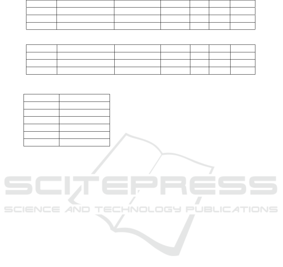
Table 6: Results obtained for the ﬁgure 6 classiﬁcation.

class imprevious surfaces Low vegetation Building Cars Trees Clutter

precision 0.93 0.95 0.86 0.9 0.81 –

Recall 0.93 0.98 0.79 0.95 0.87 –

F1-score 0.93 0.97 0.82 0.92 0.83 –

Table 7: Results obtained for the ﬁgure 7 classiﬁcation.

class imprevious surfaces Low vegetation Building Cars Trees Clutter

Precision 0.89 0.70 0.80 0.93 0.88 0.94

Recall 0.99 0.83 0.93 0.80 0.80 0.57

F1-score 0.93 0.90 0.85 0.82 0.84 0.71

Table 8: Results on the ISPRS Vaihingen dataset.

Methods Overall precision

RIT_L8 87.8%

ADL_3 88%

BKHN_9 88.8%

DLR_9 90.3%

BKHN_4 90.7%

Our result 90.2%

as an extra input channel for learning and predict-

ing, BKHN_4’s approach uses eight information from

Normalized Digital Surface Model (nDSM) and Digi-

tal Surface Model (DSM) data to learn the FCN mod-

els. Unlike these compared works, our model that

we propose in this paper remains as precise as before,

given the heterogeneity of the images.

5 CONCLUSION

CNN popularity in many computer vision tasks has

risen in the latest years and the retrieval systems for

images are not exempt from these developments. In

this paper, we proposed a DEEP HDFS framework

combined with a DEEP CNN in order to extract fea-

ture and detect objects in multi-spectral remote sens-

ing images. In our work, we have showen that even

for complex image processing tasks, a minimum of

4X velocity could be accomplished. Moreover, we

have very interesting results for the two types of

datasets, we had a precision of 90.2% for the IS-

PRS dataset and 94.2% for the multispectral dataset.

But, in the multispectral dataset, the results for the

FastH2O and the roads are very low. This can be ex-

plained as these two types look alike: two linear ob-

jects. Also, in our dataset, the number of images that

contain roads or FastH2O is not very large. So, it can

be a learning problem. In our future work, we will

focus on adapting our architecture to another type of

remote sensing data which is hyperspectral satellites

images and also we will try to ameliorate the velocity

of our approach.

REFERENCES

Almeer, M. H. (2012). Cloud hadoop map reduce for re-

mote sensing image analysis.

Basaeed, E., Bhaskar, H., Hill, P., Al-Mualla, M., and Bull,

D. (2016). A supervised hierarchical segmentation of

remote-sensing images using a committee of multi-

scale convolutional neural networks. International

Journal of Remote Sensing, 37(7):1671–1691.

Cary, A., Sun, Z., Hristidis, V., and Rishe, N. (2009). Expe-

riences on processing spatial data with mapreduce. In

International Conference on Scientiﬁc and Statistical

Database Management, pages 302–319. Springer.

Corporation, S. I. (2017). WorldView-3 Satellite Sensor

(0.31m). https://www.satimagingcorp.com/satellite-

sensors/worldview-3/.

D.Borthakur (2018a). HDFS Architecture Guide. http://

hadoop.apache.org/docs/r1.2.1/hdfs\_design.html.

D.Borthakur (2018b). MapReduce Tutorial. http://hadoop.

apache.org/docs/r1.2.1/mapred\_tutorial.html.

Donahue, J., Jia, Y., Vinyals, O., Hoffman, J., Zhang, N.,

Tzeng, E., and Darrell, T. (2014). Decaf: A deep con-

volutional activation feature for generic visual recog-

nition. In International conference on machine learn-

ing, pages 647–655.

Golpayegani, N. and Halem, M. (2009). Cloud computing

for satellite data processing on high end compute clus-

ters. In 2009 IEEE International Conference on Cloud

Computing, pages 88–92. IEEE.

Gordo, A., Almazan, J., Revaud, J., and Larlus, D. (2017).

End-to-end learning of deep visual representations for

image retrieval. International Journal of Computer

Vision, 124(2):237–254.

ISPRS (2019). SPRS Test Project on Urban Classiﬁca-

tion, 3D Building Reconstruction and Semantic La-

beling. http://www2.isprs.org/commissions/comm3/

wg4/2d-sem-label-vaihingen.html.

Jégou, S., Drozdzal, M., Vazquez, D., Romero, A., and Ben-

gio, Y. (2017). The one hundred layers tiramisu: Fully

convolutional densenets for semantic segmentation. In

Deep Semantic Feature Detection from Multispectral Satellite Images

465

Proceedings of the IEEE Conference on Computer Vi-

sion and Pattern Recognition Workshops, pages 11–

19.

Kocakulak, H. and Temizel, T. T. (2011). A hadoop solu-

tion for ballistic image analysis and recognition. In

2011 International Conference on High Performance

Computing & Simulation, pages 836–842. IEEE.

Längkvist, M., Kiselev, A., Alirezaie, M., and Loutﬁ, A.

(2016). Classiﬁcation and segmentation of satellite or-

thoimagery using convolutional neural networks. Re-

mote Sensing, 8(4):329.

Li, B., Zhao, H., and Lv, Z. (2010). Parallel isodata

clustering of remote sensing images based on mapre-

duce. In 2010 International Conference on Cyber-

Enabled Distributed Computing and Knowledge Dis-

covery, pages 380–383. IEEE.

Lv, Z., Hu, Y., Zhong, H., Wu, J., Li, B., and Zhao, H.

(2010). Parallel k-means clustering of remote sensing

images based on mapreduce. In International Confer-

ence on Web Information Systems and Mining, pages

162–170. Springer.

Marmanis, D., Wegner, J. D., Galliani, S., Schindler, K.,

Datcu, M., and Stilla, U. (2016). Semantic segmenta-

tion of aerial images with an ensemble of cnns. ISPRS

Annals of the Photogrammetry, Remote Sensing and

Spatial Information Sciences, 3:473.

Paisitkriangkrai, S., Sherrah, J., Janney, P., Hengel, V.-D.,

et al. (2015). Effective semantic pixel labelling with

convolutional networks and conditional random ﬁelds.

In Proceedings of the IEEE Conference on Computer

Vision and Pattern Recognition Workshops, pages 36–

43.

Rani, K. and Sharma, R. (2013). Study of image fusion us-

ing discrete wavelet and multiwavelet transform. In-

ternational Journal of Innovative Research in Com-

puter and Communication Engineering, 1(4):95–99.

Ronneberger, O., Fischer, P., and Brox, T. (2015). U-net:

Convolutional networks for biomedical image seg-

mentation. CoRR, abs/1505.04597.

Sun, S., Zhou, W., Tian, Q., and Li, H. (2016). Scalable ob-

ject retrieval with compact image representation from

generic object regions. ACM Transactions on Mul-

timedia Computing, Communications, and Applica-

tions (TOMM), 12(2):29.

Wang, Y., Zhang, L., Tong, X., Zhang, L., Zhang, Z., Liu,

H., Xing, X., and Mathiopoulos, P. T. (2016). A

three-layered graph-based learning approach for re-

mote sensing image retrieval. IEEE Transactions on

Geoscience and Remote Sensing, 54(10):6020–6034.

Zhang, F., Du, B., and Zhang, L. (2015). Scene classiﬁca-

tion via a gradient boosting random convolutional net-

work framework. IEEE Transactions on Geoscience

and Remote Sensing, 54(3):1793–1802.

Zhong, Y., Fei, F., Liu, Y., Zhao, B., Jiao, H., and Zhang,

L. (2017). Satcnn: satellite image dataset classiﬁca-

tion using agile convolutional neural networks. Re-

mote sensing letters, 8(2):136–145.

KDIR 2019 - 11th International Conference on Knowledge Discovery and Information Retrieval

466