Detecting Political Bias Trolls in Twitter Data

Soon Ae Chun

, Richard Holowczak

, Kannan Neten Dharan

, Ruoyu Wang

Soumaydeep Basu

and James Geller

Information Systems and Informatics at CSI, City University of New York, New York, U.S.A.

Information Systems and Statistics, Baruch College, New York, U.S.A.

Department of Computer Science, NJIT, Newark, NJ, U.S.A.

Keywords: Troll Detection, Alt-right Tweets, Political Biases, Twitter, Social Network Mining, Election Manipulation.

Abstract: Ever since Russian trolls have been brought to light, their interference in the 2016 US Presidential elections

has been monitored and studied. These Russian trolls employ fake accounts registered on several major social

media sites to influence public opinion in other countries. Our work involves discovering patterns in these

tweets and classifying them by training different machine learning models such as Support Vector Machines,

Word2vec, Google BERT, and neural network models, and then applying them to several large Twitter

datasets to compare the effectiveness of the different models. Two classification tasks are utilized for this

purpose. The first one is used to classify any given tweet as either troll or non-troll tweet. The second model

classifies specific tweets as coming from left trolls or right trolls, based on apparent extreme political

orientations. On the given data sets, Google BERT provides the best results, with an accuracy of 89.4% for

the left/right troll detector and 99% for the troll/non-troll detector. Temporal, geographic, and sentiment

analyses were also performed and results were visualized.

1 INTRODUCTION

The presence of trolls using social media to influence

politics, healthcare and other social issues has

become a widespread phenomenon akin to spam and

phishing. Ever since Russian trolls were brought to

light during the 2016 US Presidential elections, the

influence of trolls has been studied in Computer

Science and other fields. However, there is no clear

definition of what a troll is. Most authors assume that

it is obvious and their meaning of the word troll can

only be inferred from their treatment of the subject.

Mojica’s use of the word “troll” focuses on

determining the intentions of the user (Mojica, 2016),

whether the user is attempting to keep their intention

hidden, how the posts were interpreted by other users,

and what the reactions are to specific posts. Kumar et

al. (Kumar, 2014) use the term "trolling" when a user

posts and spreads information that is deceptive,

inaccurate, or outright rude. The authors developed an

algorithm called TIA, Troll Identification Algorithm,

in order to classify such users as malicious or benign.

Kumar’s study is more focused on the integrity of the

network that the trolls are working on. Thus, anyone

who posts information that is incorrect may be a troll,

unlike in (Mojica, 2016), where the intentions of a

user are the focus. In addition, if non-troll users make

negative comments or posts, they are also considered

trolls. The decision for being classified as a troll is not

only based on the users' own posts, but also on the

responses.

In our work, we focus on a subclass of trolls

defined by their domain, namely “political trolls” that

have nefarious intentions. We use machine learning

algorithms to identify Russian troll tweets. More

specifically, we employ known Russian troll tweets

(Fivethirtyeight, Roeder, 2018) to build classification

models that classify any tweet as either being from a

Russian troll or not. An initial review indicated that

not all Russian trolls are of the same kind.

Specifically, we discovered that some of the trolls

indicate a “left” political orientation, while other

trolls appear to be politically at the right end of the

spectrum. Therefore, after building a machine

learning model that distinguishes between troll and

non-troll tweets we built another model that separates

left trolls from right trolls. Figure 1 shows the overall

process flow. The box marked as Troll Classifier is

the result of running a machine learning model on

data that was already classified by humans. Similarly,

the Political Bias Classifier model has been

developed to detect the political bias towards “left” or

334

Chun, S., Holowczak, R., Dharan, K., Wang, R., Basu, S. and Geller, J.

Detecting Political Bias Trolls in Twitter Data.

DOI: 10.5220/0008350303340342

In Proceedings of the 15th International Conference on Web Information Systems and Technologies (WEBIST 2019), pages 334-342

ISBN: 978-989-758-386-5

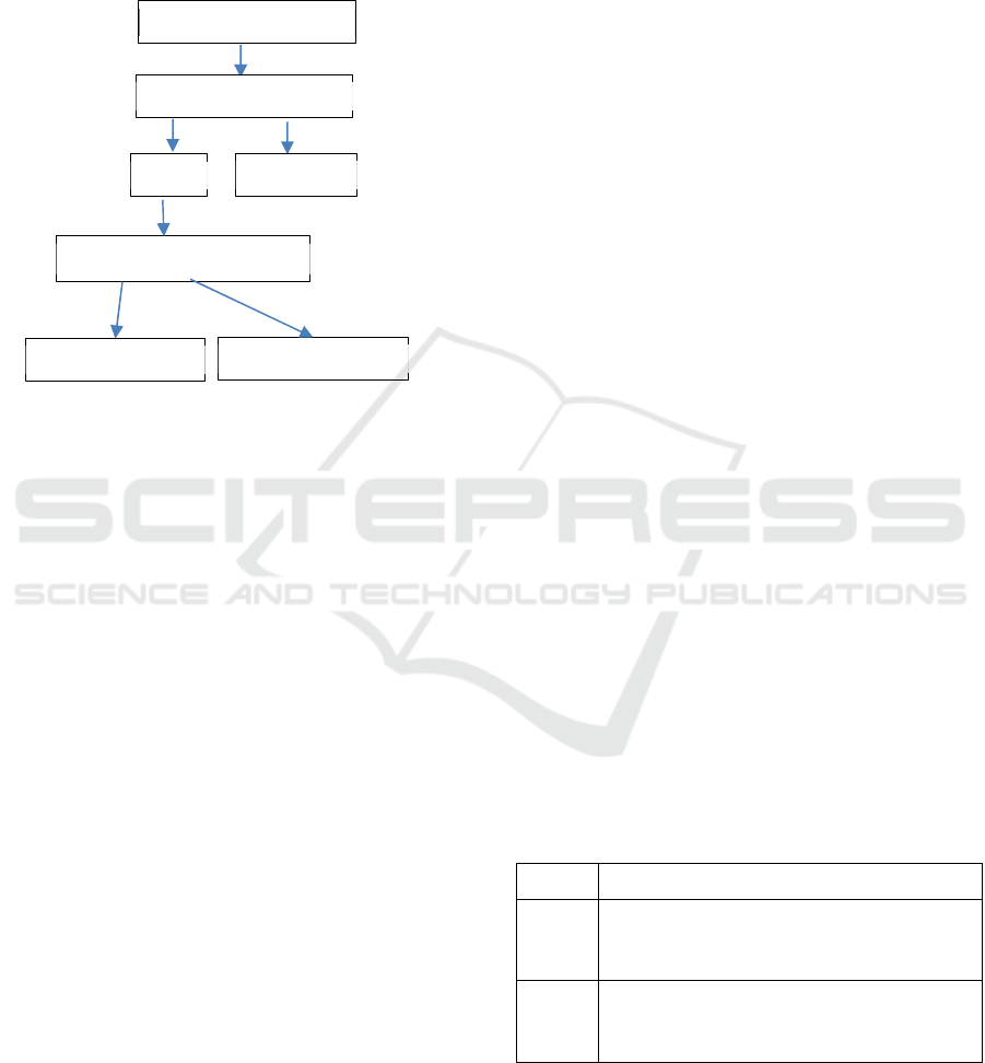
“right” orientation in the troll dataset. To analyze

whether trolls have a political bias toward one or the

other political affiliation, we use a two-step analysis.

We first identify a tweet as coming from a troll or not,

using the troll classifier and then further predict

whether it expresses a right or left bias.

Figure 1: Political Bias Troll Detection Framework.

2 DATASETS

Twitter data has been widely used in many text

mining projects. Unlike other social media platforms,

tweets are public and easy to retrieve from Twitter.

Twitter has APIs that help users to retrieve data in a

methodological way, e.g., for a specific geographic

region, a specific timeframe, etc. One can fetch data

from a targeted set of users as well.

For building our troll model and the political bias

detection model, we used a dataset published by an

online news portal called FiveThirtyEight (Roeder,

2018). This dataset contains roughly 3 million tweets

that Twitter concluded were associated with the

“Internet Research Agency (IRA).” The IRA is a

company paid by the Russian government to sow

disinformation (Wikipedia, 2019). The data is

completely open source licensed and includes

2,973,371 tweets from 2,848 Twitter handles. It

includes every tweet’s author, text and date; the

author’s follower count and the number of accounts

the author followed; and an indication of whether the

tweet was a retweet. Authors are not real names, but

fabricated personas. We call this data table the

Russian Troll dataset, where each tweet is considered

to be from a troll.

Every tweet in the data is also labeled with an

“account_type” that shows whether the tweet

indicates a left or right political orientation. Many

tweets are written in the Russian language. These

tweets have an “account_type” Russian, which we did

not consider as part of our dataset. There are over

1.538K tweets identified as “right” and

approximately 890K as having a “left” political bias.

In the first step of preprocessing, we removed

URLs. We also removed Twitter handles that

appeared to be irrelevant to the classification, and we

removed Non-ASCII characters from the tweets,

using the ‘Pandas’ package of Python (McKinney,

2017; https://pandas.pydata.org).

3 TROLL CLASSIFICATION

MODELS

The training of the troll vs. non-troll and right troll vs.

left troll classifiers was performed using different

machine learning approaches to compare their

performances. For all the machine learning

algorithms that we are using, to derive a classifier,

positive and negative instances are necessary. The

positive instances are constituted by the Russian Troll

dataset. However, we needed to generate a negative

(i.e. non-troll) data set of the same size. For this we

fetched 3 million random tweets from several Twitter

feed sites (e.g., http://followthehashtag.com/datasets/

free-twitter-dataset-usa-200000-free-usa-tweets/)

and the Tweepy API (Roesslein, 2019) to fetch real

time tweets. We labeled this dataset as “non-troll,”

hence, we will call it Non-Troll dataset.

Unfortunately, it was impossible to ascertain that

every one of these 3 million random tweets is not a

troll tweet, thus, the training data may contain some

errors. Given the very large number of tweets posted

every day (estimated at 500 million), the negative

effect should be limited.

Table 1: Sample Troll and Non-Troll Tweets.

Label Text

1 (troll)

a. Demand paper #VoteTrump #MAGA

https://t.co/YywhqRJ6DR #TrumpForPresident

b. Is Eva Braun opening for Hillary Clinton?

https://t.co/Asmktt8imd

0 (non

troll)

a. I'm at Apple Store, Pheasant Lane in Nashua,

NH https://t.co/E5FCrUFEpL

b. Super excited to continue to play basketball at

KCC next year with‚ https://t.co/QNWtA1bz08

Thus, the troll detection model was built using the

6 million tweets of the Russian Troll dataset and the

Non-Troll dataset combined together for training and

testing data.

Twitter Fee

Troll Classifier

Troll

on-Troll

Political Bias Classifier

Left Troll Twee

Right Troll Twee

Detecting Political Bias Trolls in Twitter Data

335

A tweet from the Russian Troll dataset was

assigned the label 1, while a tweet from the Non-Troll

dataset was assigned the label 0. Table 1 shows an

example of four tweets taken from the dataset, with

the label and tweet text columns, and Table 2 shows

examples of right and left political bias trolls from the

Russian Troll dataset.

In our experiments, we divided datasets into

training and test data using an 80:20 breakdown.

Table 2: Example of Left and Right biased Trolls.

Right

a. You do realize if democrats stop shooting people,

gun violence would drop by 90%

b. US sailor gets 1 year of prison for being reckless

w/ 6 photos of sub Hillary gets away w/ 33k

emails.. https://t.co/jmPjfPCRK4

Left

a. 1 dat. 4 shootings. It’s Trump’s Birthday – Tavis

Airforce Base –

b. 1 black president out of 45 white ones is the

exception that proves the rule. The rule is racism.

And then Trump came next.

3.1 Support Vector Machine Classifier

SVM (Support Vector Machines) is a popular

supervised machine learning technique (Vapnik,

1995). The Support Vector Machine conceptually

implements the following idea: input vectors are

(non-linearly) mapped to a very high-dimensional

feature space. SVM has been proven effective for

many text categorization tasks.

In SVMs, we try to find a hyperplane in an N-

dimensional space that can be used to separate the

data points with two different classifications.

“Support Vectors” define those points in the data set

that affect the position of the hyperplane. These are

the data points nearest to the hyperplane on both

sides. Usually, there are several possible hyperplanes

that can be used to classify a dataset into two different

classes. The main objective of the SVM algorithm is

to find a hyperplane with the maximum margin

between the data points. This ensures that when this

model is used to classify new data points, it is likely

to classify them correctly. It requires input data

represented as multi-dimensional vectors.

Data Preprocessing and Representation: Besides

the steps described in Section 2, we deleted emoticons

from our dataset, since we are not taking them into

consideration for building the model. For methods of

using emoticons in sentiment analysis, see, e.g.,

(Bakliwal, 2012) and our previous work (Ji, 2015).

As the next step, we applied stemming to the

dataset, using the Porter Stemmer (Porter, 2006).

To construct one input data model, we used a

Term Frequency — Inverse Document Frequency (tf-

idf) vectorizer to convert the raw text data into matrix

features. By combining tf and idf, we computed a tf-

idf score for every word in each document in the

corpus. This score was used to estimate the

significance of each word for a document, which

helps with classifying tweets.

SVM Classification Model: We built the SVM

model using the FiveThirtyEight dataset. The stored

model can be called later for classification of new

data. We used the SVM scikit-learn implementation

named SVC (Support Vector Classification). It is an

implementation based on libsvm (Chang, 2001).

In this text categorization problem, we made use

of a linear SVM classifier with the regularization

parameter, C = 0.1. The regularization parameter is

used to control the trade-off between

misclassifications and efficiency. The higher C is, the

fewer misclassifications are allowed, but training gets

slower. In our case, since our regularization

parameter is very small, misclassifications are

allowed, but training is relatively faster. As this

dataset is very large, this was necessary.

We use a Radial Basis Function (RBF) kernel for

our SVM model as the set of unique words in our data

set presents a high dimensional vector space (Albon,

2017).

3.2 Neural Network Classifier with

One-hot Encoding

Data Representation: There are two popular ways of

representing natural language sentences: vector

embeddings and one-hot matrices. One-hot matrices

contain no linguistic information. They indicate

whether words occur in a document (or a sentence)

but suggest nothing about its frequency, or itsr

relationships to other words. The creation of one-hot

matrices begins with tokenizing the sentence, that is,

breaking it into words. Then we created a lookup

dictionary of all the unique words/tokens, which need

not have a count or an order. Essentially, every word

is presented by a position/index in a very long vector.

The vector component at that position is set to 1 if the

word appears. All other components in the vector are

set to 0. For example, in a dictionary that contains

only seven words, the first word would be represented

by [1, 0, 0, 0, 0, 0, 0], the second by [0, 1, 0, 0, 0, 0,

0], etc. Each vector is of the length of the dictionary

(in our case 3000 words), and vectors are stored as

Python arrays. A whole sentence needs to be

represented by a 2-dimensional matrix.

Neural Network Classifier: For comparison with

SVM, we first built a sequential classifier, which is a

simple neural network model that consists of a stack

of hidden layers that are executed in a specific order.

WEBIST 2019 - 15th International Conference on Web Information Systems and Technologies

336

We used one dense layer and two dropout layers.

Dense neural network layers are linear neural network

layers that are fully connected. In general, in a dense

layer, every input is connected to every output by a

weight. A dense layer is usually followed by a non-

linear activation function. Dropouts are randomly

used to remove data, to prevent overfitting.

Activation functions of a node compute the output

of that node, when given any specific input or set of

inputs. The output of the activation function is then

used as the input for the next layer. Some of the most

common activation functions are ReLU (Rectified

Linear Unit), Sigmoid, SoftMax and Logistic

function. In our first input layer, we made use of the

ReLU activation function and 512 outputs come out

of that layer. Our second layer, which is a hidden

layer, consisted of a Sigmoid activation function with

256 outputs. Our output layer, consisted of SoftMax

activation functions. This configuration was the result

of a number of preliminary experiments and achieved

the best classifier performance.

We made use of a categorical crossentropy loss

function. This loss function is also called the SoftMax

loss function. It measures the performance of a

classification model, whose output is a probability

value between 0 and 1.

We used small batch sizes of 32 sentences to train

our model so that we could check its accuracy.

Smaller batches make it faster and easier to train a

model with a large dataset. We ran the algorithm for

five epochs while training, where epochs measure the

number of times the machine learning program goes

through the entire dataset during training. We

observed that six epochs led to overfitting, hence we

reverted to five epochs. We implemented the Neural

Network model using keras (Chollet, 2015) with

Tensorflow (Tensorflow, 2017) backend, which has

its own loss function and optimization function for

computing the accuracy and loss.

After the model was constructed, it was saved in

two parts. One part contains the model’s structure, the

other part consists of the model’s weights. The model

can then be used for predicting categories of tweets

on a new dataset. Results will be shown in Section 4.

3.3 CNN Neural Network Classifier

with Word2vec Representation

Data Representation: Vector embeddings are spatial

mappings of words or phrases onto a vector. In a

vector embedding a word is represented by more than

one bit set to 1. Similar patterns of 1s suggest

semantic relationships between words— for instance,

vector embeddings can be used to generate analogies.

An important vector embedding method is Word2vec

(Le & Mikolov, 2014).

Word2vec can be constructed and trained to

create word embeddings for entire documents.

Word2vec can group vectors of similar words

together into a vector space. With enough data,

Word2vec models can constrain the meaning of a

word using past appearances. The output of a

Word2vec model is a vocabulary where each item has

a vector attached to it, which can be used to query for

relationships between words.

For building our classifiers, we used an existing

Word2vec model, by the name of “Google

Word2Vec” (Skymind, 2019). It is a huge model

created by Google, which comprises a vocabulary of

about 3 million words and phrases. It was trained on

a Google news dataset of roughly 100 billion words.

The length of the vectors is set to 300 features.

Since the Word2vec representation of 3 million

words and phrases was unnecessarily large, we cut it

down to around 20,000 words, by computing the

intersection between words in our dataset and the

Word2vec model. Our embedding dimension is

equivalent to the length of the vectors, which is 300.

CNN Classifier: Convolutional Neural Networks

(CNNs) (LeCun, 1995) are a supervised machine

learning algorithm, which is mainly used for

classification and regression. CNNs usually require

very little preprocessing as compared to other neural

networks. Though CNNs were invented for analyzing

visual imagery, they have been shown to be effective

in other areas, including in Natural Language

Processing (Kim, 2014). A CNN consists of input,

output and multiple hidden layers. The intermediate

layers, which are the hidden layers, generally

comprise convolutional layers.

We used three convolutional layers other than the

input and the output layers, and we used ReLU as the

activation function for all of them. The three

sequences have the same number of filters, which is

equivalent to the total number of data points in the

training data. The filter sizes for the three

convolutional layers were 3, 4 and 5 respectively. The

activation function in the final output dense layer is

SoftMax, and the number of word embeddings is

around 20,000.

We developed CNN models with both described

data representations, one-hot encoding and

Word2Vec encoding. We trained the CNN models

over 10 epochs. We ran our model using keras with

Tensorflow backend.

Detecting Political Bias Trolls in Twitter Data

337

3.4 State-of-the-Art NLP Model BERT

BERT (Bidirectional Encoding Representations from

Transformers) (Devlin et al. 2019) applies

bidirectional training of “transformers” to language

modelling. A transformer is used for converting a

sequence using an encoder and a decoder into another

sequence. BERT is the first deeply bidirectional

model and relies on a language learning process that

is unsupervised. It has been pre-trained using only a

plain Wikipedia text corpus.

In a context-free model, the system generates a

single word embedding representation for each word

in the vocabulary, whereas previous contextual

models generated a representation of each word that

is based on other words in the sentence. However, this

was done only in one direction. BERT uses a

bidirectional contextual representation that is, it uses

both the previous and next context in a sentence

before or after a word respectively.

We made use of the BERT-base, Multilingual

Cased model with 12 layers; 768 is the size of the

hidden encoder and pooling layers and in all there are

110 Million parameters. A Cased model preserves the

true upper and lower case (cased words) and the

accent markers. Thus “bush” (the shrub) is different

from “Bush” (the president). We trained our model

for three epochs with a batch size of 32 and sequence

length of 512. The learning rate was 0.00002. As

before we used keras with Tensorflow.

The max_position embedding was set to 512,

which is the maximum sequence length. That means

that a specific tweet can have a maximum length of

512 characters. Everything beyond 512 characters is

ignored. The num_attention_heads parameter was set

to 12, which is the 12-head attention mechanism. In

this mechanism, the vector is split into 12 chunks,

each having a dimension of 512/12 = 42 (42.666…)

and the algorithm uses these chunks for each attention

layer in the Transformer encoder. Exhaustive

experiments with these hyperparameters is practically

impossible, but the chosen parameters provided the

relatively best results in our experiments.

We made use of an Adam optimizer, which is the

default optimizer for BERT. Adam is an alternative to

Stochastic Gradient Descent (SGD), which is used to

update network weights iteratively when training

with data. A learning rate is maintained for each

network weight (parameter) and separately adapted as

learning unfolds. The model was saved for future use

for classification and was also evaluated.

3.5 Political Bias Classifiers

To classify the political orientation of tweets, we

trained the corresponding models described in

Sections 3.1—3.4, based on the Russian Troll dataset.

The Russian Troll dataset has a field labeled

“account_type” with the political bias or orientation

values of left or right (among others).

The right and left political orientation data

distribution in the Russian Troll dataset used for

training and testing is as follows: Right: 1,538,146;

Left: 890,354. The SVM, Fully Connected NN, and

CNN models and the BERT-encoded CNN model

were used to classify the left and right political bias

in a tweet.

4 RESULTS

4.1 Political Bias Troll Detection

Models

Table 3 compares the accuracy, precision and recall

scores for the troll detection and political bias

detection models. It shows that the neural network

models (fully connected NN and CNN models)

performed worse than the base SVM model. On the

other hand, the BERT model outperformed all other

models with an accuracy level of 99%, and with

precision and recall levels of 98% and 99%

respectively.

Table 3: Comparing the accuracy, precision and recall of

five Machine Learning Models.

Model

Classifier Type

Accuracy Precision Recall

SVM

Model

Troll Detector 84% 85% 86%

Political Bias

Detecto

86% 88% 91%

NN with

One-hot

Encoding

Troll Detector 74% 76% 76%

Political Bias

Detecto

84% 88% 90%

CNN with

One-hot

Encoding

Troll Detector 74% 78% 81%

Political Bias

Detector

84% 85% 86%

CNN with

Word2-vec

Troll Detector 56% - -

Political Bias

Detecto

85% - -

BERT

model

Troll Detector 99% 98% 99%

Political Bias

Detecto

89% 89% 90%

An important drawback of one-hot encoding is that it

increases the length of the data vectors. We used only

the 3000 most commonly occurring words in the

WEBIST 2019 - 15th International Conference on Web Information Systems and Technologies

338

training corpus, and hence each one-hot vector is of

dimension 3000. The performance of CNN with the

Word2vec model is significantly lower than that of

the SVM, NN or CNN with one-hot encoding models,

with an accuracy level of only 56%.

For political bias classification experiments, the

accuracy of SVM, 86%, was slightly better than NN

or CNN with one-hot encoding and CNN with

Word2Vec, with accuracies of 84%, 84% and 85%,

respectively. However, the BERT-based

classification model again outperformed the others

with an accuracy level of 89%.

4.1.1 Political Bias Troll Analysis in Tweets

We collected a new unique data set of tweets starting

in October of 2016, just prior to the US election. An

initial set of 500 Twitter handles belonging to “Alt-

Right,” "Right,” “Right-Center,” “Left-Center,” and

“Left” biased magazines, web sites and personalities

was identified using data collected from the Media

Bias/Fact Check web site (Media Bias/Fact Check).

The initial set of Twitter handles was thus labeled

with biases as follows:

Alt-Right Bias: 103 twitter handles

Right Bias: 133 twitter handles

Right Center Bias: 77 twitter handles

Left-Center Bias: 122 twitter handles

Left Bias: 65 twitter handles

The Alt-right bias media sources are often described

as moderately to strongly biased toward conservative

causes, through story selection and/or political

affiliation. They often use strong, “loaded” words to

influence an audience by using appeals to emotion or

stereotypes, publish misleading reports and omit

reporting of information that may damage

conservative causes.

We next identified followers of each of these

Twitter handles (eliminating duplicates) and then

proceeded to download their complete tweet histories,

thus including tweets from many years back. Each

tweet was then labeled with the Twitter handle and

political bias. The results of the data collection

include 1.6 billion tweets from 25 million unique

Twitter handles. Random samples of 1 million, 5

million and 20 million tweets were extracted to form

the data set for further analysis. We call these samples

Political Bias datasets, and we applied our model to

classify them into trolls vs. non-trolls.

The SVM models were used on the Political Bias

1 million tweet dataset and the results are in Table 4.

Among 1 million tweets, 730,215 are considered

trolls and among these, the right trolls (546,430)

outnumber the 183,785 left trolls. When the CNN

neural network classification model with one-hot

matrices representation was applied to the 5 million

tweets, over 3,586K tweets were classified as trolls.

Among these, the right troll set consisted of 2,553K

tweets, outnumbering the left trolls (1,032K tweets),

as shown in Table 4.

Table 4: Political Bias trolls using SVM and CNN with one-

hot encoding and two classifier models.

Tweet Type SVM CNN

Sample datase

1000000 5000000

Troll Tweets 730215 3586213

Left Troll Tweets 183785 1032422

ht Troll Tweets 546430 2553791

Thus, 75% and 71% of all troll tweets were found to

be politically right tweets, compared to left tweets

(25% and 29%) for the respective models.

We applied the BERT-encoded CNN model for

classifying the 5 million tweet Political Bias dataset

into troll vs. non-troll tweets. The results show that

3,598,898 (72%) were trolls and 1,401,102 (28%)

were non-trolls. The breakdown of Political Bias

tweets into trolls and non-trolls is shown in Table 5.

Table 5: Political biases in non-troll tweets and troll tweets

using BERT -CNN Classification Model.

on-Trolls Trolls

AltRi

530,990 2,013,935

31,897 64,533

htCente

162,061 330,314

eutral 492,820 766,660

LeftCente

122,681 270,755

Lef

60,653 152,701

Table 6: Average Number of Troll tweets and % of Trolls

by Political Bias of Unique Tweet handles.

Poltical Biases

# of

tweethandles

Avg # of

Troll tweets

% of Trolls

AltRight 541 1098 76%

Right 29 530 2%

RightCenter 78 789 8%

Neutral 189 393 10%

LeftCenter 43 595 3%

Left 37 180 1%

Grand Total 917 844 100%

We identified 917 unique Twitter handles (users) that

were associated with trolls from the 1 million tweet

machine-labeled dataset, as shown in Table 6, using

BERT classifiers. A much higher average number of

troll tweets (on average 1098 tweets per unique

handle, 76% of all trolls) were associated with the 541

Detecting Political Bias Trolls in Twitter Data

339

unique Twitter handles with an alt-right bias, while a

total of 80 user accounts considered as left center or

left posted on average 595 (3%) and 180 (1%) troll

tweets, respectively.

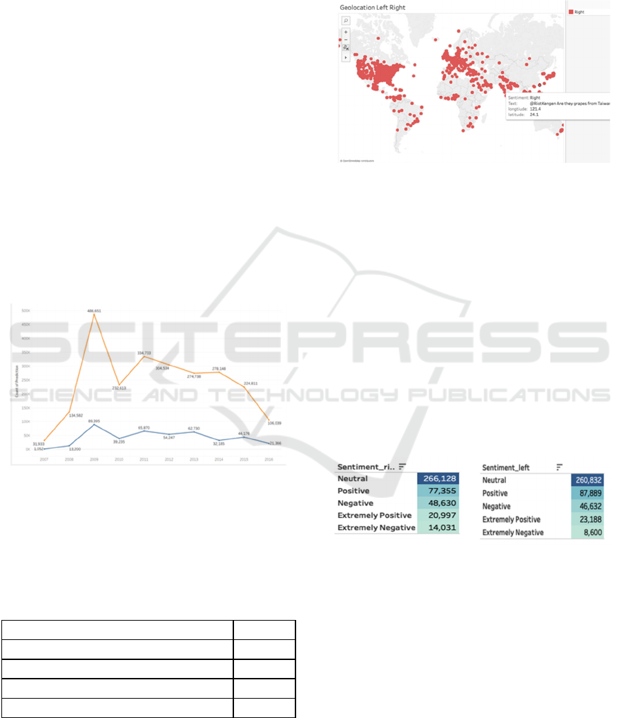
4.2 Temporal Analysis

We performed a temporal progression analysis of left

and right trolls after identifying trolls using the 5

million Political Bias sample dataset to understand

how political bias troll tweets have changed over

time. Figure 2 shows the temporal analysis from 2004

to 2016. In 2009, there was a notable peak of trolls,

especially right-biased trolls. This coincides with the

beginning of Barak Obama’s first presidency.

4.3 Geospatial Analysis

We performed a geospatial analysis on 5 million

tweets to locate the left and right troll tweets. In the

dataset, only 133,801 tweets (2.7%) had geolocation

information and 83,232 geolocated tweets were

classified as trolls. Table 7 shows the number of left

and right troll tweets based on the geolocation data.

Figure 2: Temporal Analysis on Political Bias Trolls: Blue

= Left Trolls. Yellow = Right Trolls.

Figure 3 show the geospatial distribution of approx.

50K right troll tweets. The distribution of left troll

tweets is omitted due to space constraints.

Table 7: Breakdown of tweets containing geo location

information from the 5 Million tweets dataset.

Tweet type (from 5 Million) Count

Total tweets with geolocation 133801

Total Troll Tweets with geolocation 83232

Right Trolls with geolocation 50154

Left Troll with geolocation 33078

The total ratio of right to left troll tweets is 60:40 in

Japan, South Korea and Thailand, where the right

troll tweets are more prominent. In the UK, the count

of left troll tweets is significantly higher as compared

to the right troll tweets. In the United States, the ratio

of left to right troll tweets is 60:40. We also observe

that the right troll tweets and left troll tweets are

evenly distributed in most of the countries.

Figure 3: Geospatial distribution of Right troll tweets.

4.4 Sentiment Analysis on Political Bias

Dataset of Five Million Tweets

Sentiment analysis was performed for left and right

troll tweets to understand the emotional tone that

trolls used to influence people’s minds. The sentiment

analysis model was built using the Sentiment140

dataset (Sentiment140)

Figure 4 illustrates the breakdown of sentiments

of right troll tweets, which have been classified into

five different classes, namely neutral, positive,

extremely positive, negative and extremely negative,

based on the data. Figure 5 shows the same

breakdown for left troll tweets. Figure 6 shows a side-

by-side comparison.

Figure 4: Sentiments of

right bias trolls.

Figure 5: Sentiments of

left bias trolls.

The sentiment analysis results show the following:

 The ratio of positive, negative and neutral trolls

does not vary much in either left or right troll

tweets.

 The number of negative tweets is slightly higher

in right troll tweets by a count of around 7,000

tweets.

 The number of positive tweets is slightly lower in

right troll tweets by a count of 13,000 tweets.

WEBIST 2019 - 15th International Conference on Web Information Systems and Technologies

340

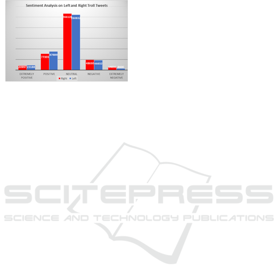
Figure 6: Sentiment analysis on right (in red) and left (blue)

troll tweets.

5 CONCLUSIONS AND FUTURE

WORK

In this paper, we built several machine learning

models to identify the political bias of trolls. The

classifiers for troll identification were developed with

the Russian Troll dataset. The BERT-encoded

classification models had an accuracy of 89.4% for

left/right troll detector and 99% for troll/non-troll

detector, which is higher than SVM, CNN with

Word2vec and Neural Network with one-hot

encoding. Using the troll detection and political bias

detection models, we analyzed the large scale

Political Bias datasets of varying sizes. There are

more Alt-right accounts/users associated with large

numbers of troll tweets in the number of trolls and

total proportion of trolls than left biased users. We

also presented geospatial, temporal and sentiment

analyses. Sentiment analysis on the Political Bias

tweets shows that there are slightly fewer positive

right troll tweets compared to left troll tweets.

In future work, we plan to develop a large-scale

web-based system that performs real time

classification of political bias trolls to monitor the

trolls and their political biases and to perform the

geospatial and temporal analyses for identifying

extreme political bias regions and time intervals. We

also plan to perform troll contents analyses to

understand the topics and topic categories of trolls of

different political affiliations. Lastly, we want to

extend our methods to other social networks, such as

Reddit, following work by Weller and Woo (2019).

ACKNOWLEDGEMENTS

This work is partially supported by NSF CNS

1747728 and

1624503, and by the National Research

Foundation of Korea Grant NRF-2017S1A3A2066084

It is supported by PSC-CUNY Research Awards

(Enhanced): ENHC-48-65. 2017-2018.

This research was supported, in part, by the City

University of New York High Performance

Computing Center at the College of Staten Island

financed in part by National Science Foundation

Grants CNS0958379, CNS-0855217, ACI-1126113.

REFERENCES

Mojica, L. G., 2017. A Trolling Hierarchy in Social Media

and a Conditional Random Field for Trolling Detection,

arXiv:1704.02385v1 [cs.CL].

Kumar, S., Spezzano, F., Subrahmanian, V.S., 2014.

Accurately detecting trolls in slashdot zoo via

decluttering. In Proc. of the 2014 International

Conference on Advances in Social Network Analysis

and Mining, ASONAM ’14, 188–195, Beijing, China.

Vapnik, V. 1995. Support-Vector Networks, Machine

Learning, 20, 273-297.

Kim, Y. 2014. Convolutional Neural Networks for

Sentence Classification, Proceedings of the 2014

Conference on Empirical Methods in Natural Language

Processing (EMNLP), pages 1746–1751. Also in:

arXiv:1408.5882v2 [cs.CL].

LeCun, Y. 1995. Convolutional Neural Networks for

Images, Speech, and Time Series, arXiv:1408.5882v2

[cs.CL].

Chang, C.-C., Lin, C.-J., 2011. LIBSVM: A Library for

Support Vector Machines, ACM Transactions on

Intelligent Systems and Technology (TIST), Volume 2

Issue 3.

Roeder, O., 2018. Why We’re Sharing 3 Million Russian

Troll Tweets https://fivethirtyeight.com/features/why-

were-sharing-3-million-russian-troll-tweets/, Retrieved

June 3, 2019.

Fivethirtyeight, Russian-troll-tweets, https://github.com/

fivethirtyeight/russian-troll-tweets/ Retrieved in Jan

2019.

Wikipedia contributors, 2019. Internet Research Agency. In

Wikipedia, The Free Encyclopedia. https://

en.wikipedia.org/w/index.php?title=Internet_Research

_Agency&oldid=900092717, Retrieved June 3, 2019.

McKinney, W., 2017. Python for Data Analysis, 2nd

Edition -- Data Wrangling with Pandas, NumPy, and

IPython. O'Reilly Media.

Roesslein, J., 2019. https://tweepy.readthedocs.io/en/latest,

https://github.com/tweepy/tweepy, Retrieved June 3,

2019.

Bakliwal, A., Arora, P., Madhappan, S., Kapre, N., Singh,

M., Varma, V., 2012. Mining Sentiments from Tweets.

3rd Workshop on Computational Approaches to

Subjectivity and Sentiment Analysis, pages 11–18.

Detecting Political Bias Trolls in Twitter Data

341

Ji, X., Chun, S., Wei, Z., Geller, J., 2015. Twitter sentiment

classification for measuring public health concerns.

Social Network Analysis and Mining. Issue 1/2015.

Porter, M., 2006. The Porter Stemming Algorithm.

https://tartarus.org/martin/PorterStemmer/, Retrieved

June 3, 2019.

Albon, C, 2017. SVC Parameters When Using RBF Kernel,

https://chrisalbon.com/machine_learning/support_vect

or_machines/svc_parameters_using_rbf_kernel/,

Retrieved June 3, 2019.

Chollet, F., et al., 2015. Keras: The Python Deep Learning

library, https://keras.io/, Retrieved June 3, 2019.

Le, Q., Mikolov, T., 2014. Distributed Representations of

Sentences and Documents, Proceedings of the 31st

International Conference on Machine Learning,

Beijing, China, JMLR: W&CP volume 32.

Skymind. A Beginner's Guide to Word2Vec and Neural

Word Embeddings, https://skymind.ai/wiki/word2vec,

Retrieved June 3, 2019.

Tensorflow, 2017. https://www.tensorflow.org/, Retrieved

June 3, 2019.

Devlin, J., Chang, M.W., Lee, K., Toutanova, K., 2019.

BERT: Pre-training of Deep Bidirectional

Transformers for Language Understanding,

https://arxiv.org/pdf/1810.04805.pdf, Retrieved June 3,

2019.

Weller, H., and Woo, J. 2019. Identifying Russian Trolls on

Reddit with Deep Learning and BERT Word

Embeddings. http://web.stanford.edu/class/

cs224n/reports/custom/15739845.pdf, Retrieved June

12, 2019.

Sentiment140: dataset with 1.6 million tweets -

https://www.kaggle.com/kazanova/sentiment140.

Media Bias/Fact Check, https://mediabiasfactcheck.com/,

Retrieved June 3, 2019.

WEBIST 2019 - 15th International Conference on Web Information Systems and Technologies

342