
Restart Operator for Optimization Heuristics in Solving Linear
Dynamical System Parameter Identification Problem
Ivan Ryzhikov
1,2 a
and Christina Brester
1,2 b
1
Department of Environmental and Biological Sciences, University of Eastern Finland, Kuopio, Finland
2
Institute of Computer Science and Telecommunications, Reshetnev Siberian State University of Science and Technology,
Krasnoyarsk, Russia
Keywords: Dynamical System, Restart, Heuristics, Meta-heuristics, Parameter Identification, Evolutionary Algorithm,
Bio-inspired Algorithms.
Abstract: In this study, the parameter identification problem for linear dynamical systems is considered. The system is
assumed to be represented as a linear differential equation in general form, so the right-hand side equation
contains input function and its derivatives. This problem statement extends the order reduction problem,
where we need to find the equation of the lower order to approximate the real system output observations.
Considered problem is reduced to an optimization one. The reduced problem is complex, and we propose the
combination of stochastic optimization algorithm and restart operator. This operator aim is to prevent the
algorithm stagnation by starting the search over again if no remarkable solution improvement is detected or
if algorithm searches in the area where stagnation had been detected.
1 INTRODUCTION
In this paper, we consider parameter identification
problem for dynamical system and its approach using
optimization heuristic with specific operator that
controls the search. Dynamical system parameter
identification problems (Ramsay and Hooker, 2017)
are complex and appears in different application
fields (Gennemark and Wedeling, 2009). The main
idea is to identify the parameters of the differential
equation so its solution would fit the observation data
the most. We assume that we know the degrees of the
left-hand side and right-hand side equations and
initial point of the dynamical system. The problem of
parameter identification for the differential equation
of the second order finds plenty of applications and is
considered in different studies. In most of them, the
evolution-based algorithms are applied to solve the
reduced identification problem: genetic algorithm
(Parmar and Prasad, 2007), big bang big crunch
(Desai and Prasad, 2011) and cuckoo search (Narwal
and Prasad, 2016). In this case, the considered
approach generalizes the order reduction problem so
that any of possible degree, both state and input
a
https://orcid.org/0000-0001-9231-8777
b
https://orcid.org/0000-0001-8196-2954
variables. There are also studies on identification of
the single output dynamical system parameters, when
the right-hand side equation is just the control
function. That means, that considered in this study
approach extends the class of dynamical systems by
adding the input derivatives to the right-hand side
equation.
Many of optimization algorithms utilized to solve
real world problem are stochastic. There are different
implementations of the general idea on how the
natural systems evolve. However, what all these
algorithms have in common is exploration of the
searching space and seeking for the better alternative.
There are plenty of adaptation schemes and
algorithms interaction schemes, which allow
increasing searching performance. Also, there are
plenty of problem-oriented modifications, which
improve performance for optimization problems.
This study focuses on pairing algorithm with
restart operator for solving identification problem. In
that sense, we develop a heuristic that is applicable
for different algorithms despite of their basic idea and
its implementation. Proposed restart heuristic
identifies and prevents algorithm stagnation by
252
Ryzhikov, I. and Brester, C.
Restart Operator for Optimization Heuristics in Solving Linear Dynamical System Parameter Identification Problem.
DOI: 10.5220/0008495302520258
In Proceedings of the 11th International Joint Conference on Computational Intelligence (IJCCI 2019), pages 252-258
ISBN: 978-989-758-384-1
Copyright
c
2019 by SCITEPRESS – Science and Technology Publications, Lda. All rights reserved

starting another search if the algorithm is trapped in a
local optimum area or in the area that was found in
previous runs. Stagnation happens when algorithm
cannot get out of the local optimum area and at the
same time cannot sufficiently improve the best
alternative in it. Here we assume that another
algorithm launch would at least explore the search
space more.
The so-called restart operator checks if any
statistic exceeds predefined limitation. If it happens
than the search starts over again, so, probably another
optimum will be found. This operator improves the
optimization algorithm performance for some
optimization problems. It can be also applicable for
managing the computational resources in multiple
runs of stochastic algorithms. That approach has
some benefits in solving time-consuming problems,
where the exploration is critical, and the global
optimum is hard to be found.
To investigate the algorithm performances with
and without the restart operator, we examine
optimization algorithms on a set of data samples,
produced by different dynamical systems. All
examples are considered noiseless ones.
2 IDENTIFICATION PROBLEM
In this chapter, we consider the dynamical system
identification problem. First, we discuss the
mathematical model of the dynamical system and
then suggest the way to calculate the objective
function. Objective function appears when we reduce
the problem to the unconstrained global optimization
problem on the real vector space.
2.1 Model
Let the system model be described with the linear
differential equation:
,
(1)
where
and
are
the model coefficients, is the system state and is
the system input, and are the maximum degrees
of the system output and the system input,
respectively. We consider systems where the output
is observable and the input is known.
Since and are the highest degrees, then
parameter
, so we can simplify (1):
.
(2)
Now the model can be described with equation (2)
and the model output on input can be found by
solving the Cauchy problem:
(3)
where is the vector of initial values. The equation
(2) is time invariant; by that reason, we assign initial
time point as 0 in (3). In this research we also assume
that .
We solve considered Cauchy problem (3) for
equation (2) numerically with Runge-Kutta
integration scheme.
2.2 Objective Function
Let us denote the parameters we need to identify as
and
. The
system observation data is
and
observation times is
, where is
the sample size. In this study, without loss of
generality, we assume that the observation times are
the same as integration time points. The last means
that the solution of (3) at time
is
. We also
assume that we know the initial point and the input
function .
Now we can reduce the identification problem to
the optimization problem, in which we need to
minimize the objective function:
,
(4)
where
is the solution of the Cauchy problem (3)
for given and
parameters and the difference
between
and is used here for scaling
the error. The scaling of the error statistics provides
better interpretation of the real error between the
solution and observation data.
In general, objective function (4) is complex,
multimodal and requires the global optimization
approach to find the parameters that reach the
extremum of function.
We use specific fitness function for the
evolution-based optimization algorithms:
,
(5)
where function
, and the greater this
function is, the better solution is. This fitness function
will be used in further examination of the results.
Restart Operator for Optimization Heuristics in Solving Linear Dynamical System Parameter Identification Problem
253

3 SOLVING REDUCED
PROBLEM
We propose applying stochastic search heuristic
combined with restart operator for solving the
reduced problem formulated in (4). Standard and
common optimization heuristics were applied.
Algorithms and details of their implementation are
considered below. The restart operator was designed
on the basis of (Ryzhikov et al., 2016).
3.1 Optimization Algorithms
As the main optimization algorithms, the real-value
genetic algorithm, differential evolution algorithm
and particle swarm optimization were used.
The settings of the algorithms were the following:
200 or 500 iterations and 100 alternatives in iteration.
The initial population is uniformly distributed on
. The optimization problem is considered
as unconstrained, so there are no boundaries for the
variables during the search.
Real value genetic algorithms has tournament
selection with tournament size equal to 10. We used
2-parent uniform crossover, where each variable of
the offspring is taken randomly from one of its
parents, according with the scheme of uniform
crossover in evolutionary strategies (Beyer and
Schwefel, 2001). The mutation is implemented by the
following scheme:
,
(6)
where is a variable chosen in alternative that is
processed by the mutation operator,
is mutation
probability,
is uniformly generated value on
and
is randomly generated value on
.
Real value genetic algorithm is combined with
local optimization, where for randomly chosen 10
alternatives we chose the variable also randomly and
make a step of 0.1 to random direction. If after this
step we discover a better solution, we substitute the
current one with the new one.
Differential evolution algorithm is applied in its
standard form (Storn and Price, 1997). The crossover
probability is set as 0.2 and the differential weight is
1.4. The parameter values were chosen according to
brief investigation of the algorithm performance for
the current problem.
Particle swarm optimization algorithm is also
applied in its standard form (Kennedy and Eberhart,
1995), with
and
. The reason for
that choice of parameters is the same as for the
differential evolution algorithm.
3.2 Restart Operator
The restart operator checks the stagnation via the
following inequality:
,
(7)
where
is the best fitness value ever found by the
algorithm in the current run by the i-th
iteration,
is the best fitness value by the
-th iteration,
is a restart window size and
is a
threshold. So, if the difference between best fitness
values does not change sufficiently (does not exceed
) for the last
iterations, it is decided to start the
algorithm again.
If we do the restart, we also keep the best
alternative found by the algorithm. So if the best
solution in another run is close to the one found
earlier, we also do the restart. According to that, there
is another condition to check:
,
(8)
where
is the set of alternatives, which was found
by the algorithm by the time when the restart initiated
and
is the best alternative found in the current
algorithm run by the i-th iteration,
is another
restart operator parameter.
4 EXAMINATION
For examination of the algorithm performance we
considered differential equations given in the Table 1.
These equations were had been used to generate the
sample on the time interval
and then we took
200 points out of each solution. As a control function
we used
.
Table 1: Parameters for identification problems.
Number
Parameters
1
2
3
ECTA 2019 - 11th International Conference on Evolutionary Computation Theory and Applications
254
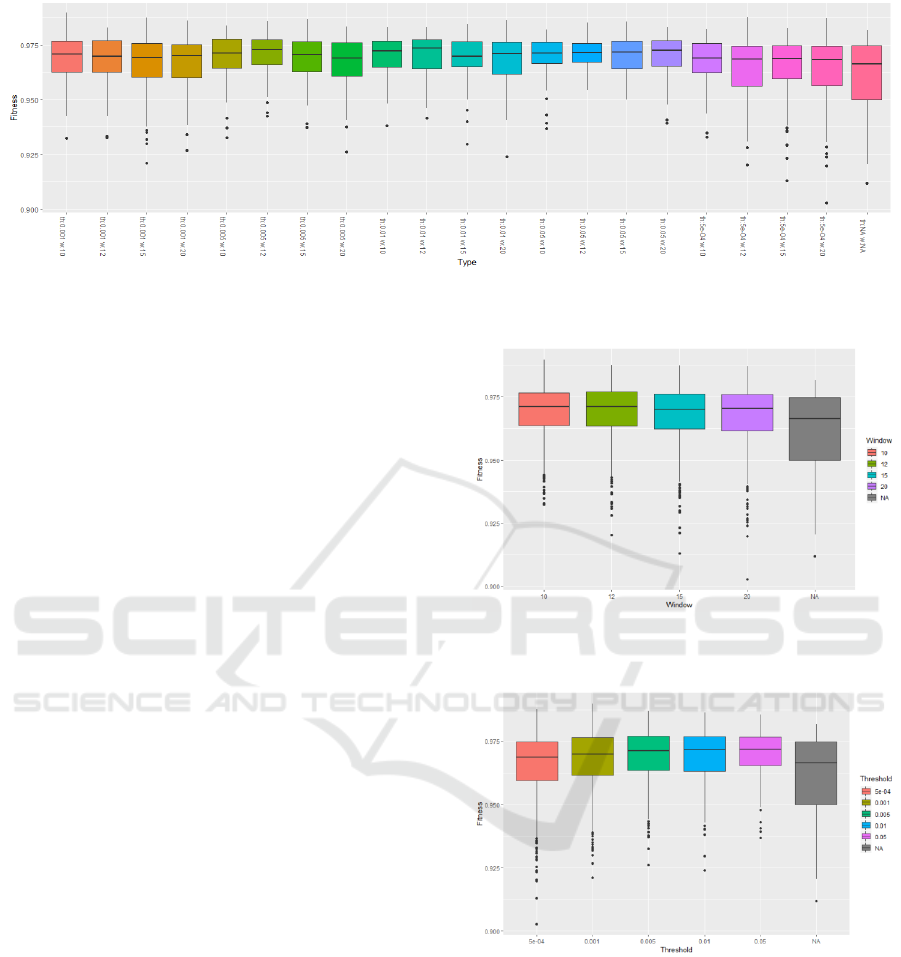
Figure 1: Best fitness value boxplot for different settings: window size + threshold. Statistic for the algorithm without restart
operator is on the right. Problem 1 from the Table 1 solved by real-valued genetic algorithm with 200 iterations.
First, let us apply the real-valued genetic
algorithms with restart operator and 200 iteration
search to all of these problem and for the following
restart operator parameters:
,
and
. We considered all the combinations
of these parameters and made 40 independent
launches of the algorithm. For the first experiment we
take the problem number 1 from the Table 1.
In Figure 1 one can see the boxplot of the fitness
values of the best solutions found by algorithms for
40 runs. In that figure, one can see the performance
of different combinations of the restart parameters:
window size and threshold. The box on the right
represents the statistic for the algorithm without the
restart operator. All the cases with restart operator
outperform the standard algorithm, since the majority
of the fitness values and their median value is closer
to 1.
All the Figures have the statistic for standard
algorithm represented on the right. The legend or axis
labels named NA means that the parameter is missing
and so the statistic represents the algorithm without
the restart operator. Boxplots are represented in their
common way.
In Figures 2, 3 and 4 one can see the fitness
boxplots for various values of the restart parameters:
window size
, threshold
and distance
,
respectively.
All the figures prove that different settings of the
restart outperform the standard algorithm. We also
can say that the threshold is the parameter is the most
influencing one.
Now let us examine the same algorithm for the
problems 2 and 3 from the Table 1 and make the same
tests for that problem. Boxplots that show how
different combinations of threshold and window size
affect the algorithm performance is given in Figure 5
and in Figure 6.
Figure 2: Fitness values boxplot for different restart
window sizes.
Figure 3: Fitness values boxplot for different restart
threshold parameter values.
Figure 5 we can see some settings, which make
algorithm not as efficient as its standard
implementation. The situation shown in Figure 6 is
worse. For problem 3 the standard algorithm
outperforms most of the algorithms with the restart
operator. But here we can see the trend: algorithms
with restart with small window size are not worse
than the original algorithm.
Restart Operator for Optimization Heuristics in Solving Linear Dynamical System Parameter Identification Problem
255
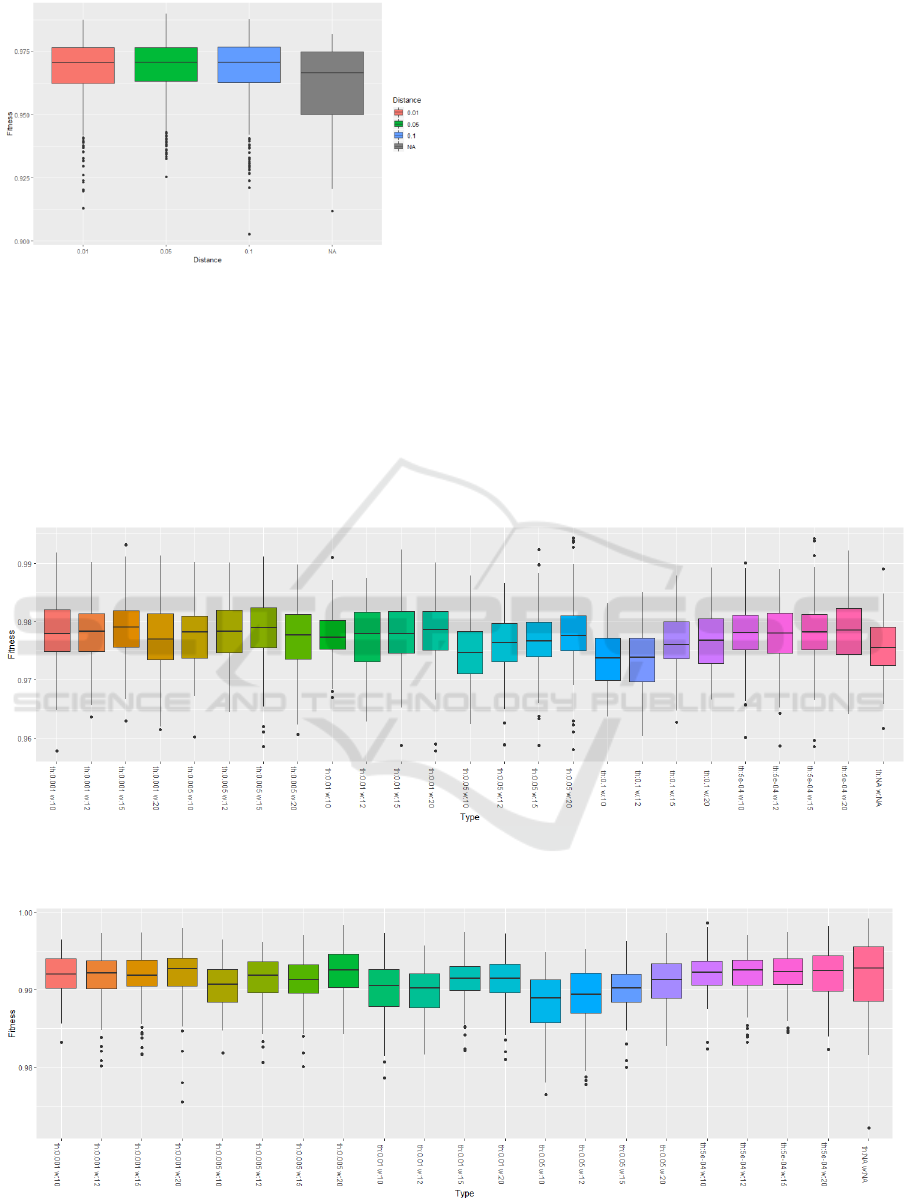
Figure 4: Fitness values boxplot for different distances.
The further investigation would be based on
solving problem 1 from the Table 1. First of all, let us
check what if we increase the number of objective
function calculations to 500. To make the results
clearer here we use the window size equal 15,
distance to 0.01 and vary only the thresholds. The
similar boxplots are presented on the Figure 7.
Starting from here we will consider the following
values for the restart threshold:
.
Increasing the computational resources for the
original algorithm caused an increase of its
performance, so it became much closer to the
algorithms with restart and even outperformed some
of its settings. But if we look at the Figure 1, we will
see that algorithms with smaller resources have the
same efficiency.
What if we use the half of the computational
resources for hybridization of the real-valued genetic
algorithm with a local search? The boxplots are given
in Figure 8, where it is shown that combination of the
local search and restart increased the overall
efficiency.
The further investigation will be provided for
differential evolution algorithm and particle swarm
optimization for solving problem 1 with 500
iterations. For these algorithms we consider windows
equals 15 and 75. The similar boxplots for differential
evolution are given in Figure 9 and Figure 10.
Figure 5: Best fitness value boxplot for different settings: window size + threshold. Statistic for the algorithm without restart
operator is on the right. Problem 2 from the Table 1 solved by real-valued genetic algorithm with 200 iterations.
Figure 6: Best fitness value boxplot for different settings: window size + threshold. Statistic for the algorithm without restart
operator is on the right. Problem 3 from the Table 1 solved by real-valued genetic algorithm with 200 iterations.
ECTA 2019 - 11th International Conference on Evolutionary Computation Theory and Applications
256
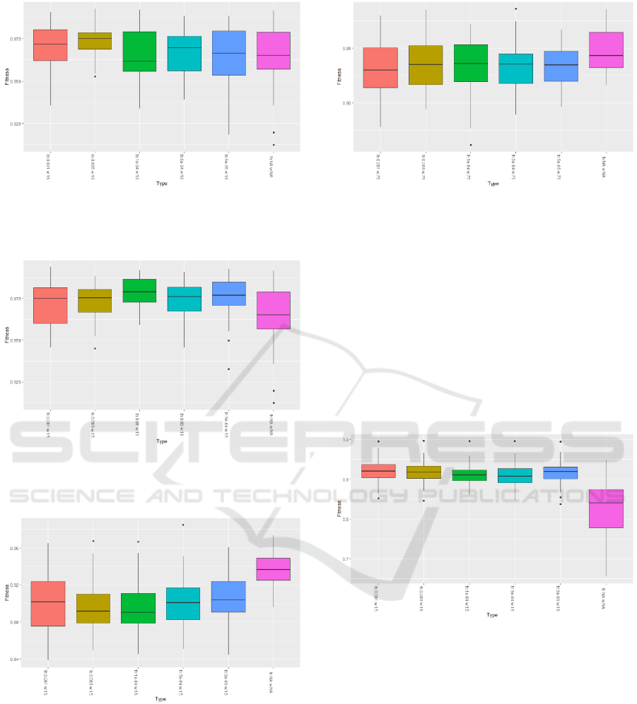
Figure 7: Fitness values statistics for different restart
parameters. Problem 1 from the Table 1 solved by real-
valued genetic algorithm with 500 iterations.
Figure 8: Fitness values statistics for different restart
parameters. Problem 1 from the Table 1 solved by real-
valued genetic algorithm with local search.
Figure 9: Fitness values statistics for different restart
parameters. Problem 1 from the Table 1 solved by
differential evolution, window size is 15.
Figure 9 shows that restart does not improve the
performance of the differential evolution algorithm
for solving the considered problem. One can also see
that the differential evolution performance is much
lower than the real-value genetic algorithm’s one.
Figure 10: Fitness values statistics for different restart
parameters. Problem 1 from the Table 1 solved by
differential evolution, window size is 75.
Figure 10 shows that increasing the window size
make the algorithm behaviour closer to the original
algorithm, as it was expected. According to Figure 10
and Figure 3 there are problems for which restart
operator does not improving the performance of the
differential equation parameters search.
Let us do the same experiments for the particle
swarm optimization algorithm. The boxplot diagrams
for window size equal 15 and 75 are given in Figure
11 and Figure 12, respectively.
Figure 11: Fitness values statistics for different restart
parameters. Problem 1 from the Table 1 solved by particle
swarm optimization, window size is 15.
Figure 11 shows that particle swarm optimization
algorithm is outperformed by the real-valued genetic
algorithm and differential evolution. But at the same
time, we can see that restart sufficiently improved its
performance and the maximum fitness value is even
close to 1.
Increasing the window size has the same effect as
for the differential evolution. Restart performance is
getting closer to the original algorithm’s one.
Restart Operator for Optimization Heuristics in Solving Linear Dynamical System Parameter Identification Problem
257

Figure 12: Fitness values statistics for different restart
parameters. Problem 1 from the Table 1 solved by particle
swarm optimization, window size is 75.
5 CONCLUSIONS
In this study we considered parameter identification
problem for the linear dynamical models. This
problem differs from the other parameter
identification problems because it is assumed that the
right-hand side equation contains input function and
its derivatives.
The considered problem is complex and
multimodal and requires a specific approach. This is
proven by the low efficiency of particle swarm
optimization and differential evolution algorithms
applied to this problem.
In this work, an operator is proposed that can
improve the algorithms’ performance preventing its
stagnation. But this operator has different effect on
different optimization algorithms: it improved the
genetic algorithm and particle swarm optimization
algorithm but decayed the differential evolution
performance. We can also conclude that the restart
operator is parameter sensitive.
The goal of the further research is to explore other
heuristics to improve the algorithms efficiency in
solving linear dynamical system parameter
identification problem.
ACKNOWLEDGEMENTS
The reported research was funded by Russian
Foundation for Basic Research and the government of
the region of the Russian Federation, grant № 18-41-
243007.
REFERENCES
Beyer, H.-G., Schwefel, H.-P, 2002. Evolution Strategies:
A Comprehensive Introduction. Journal Natural
Computing, 1(1):3–52.
Desai, S., Prasad, R., 2013. A novel order diminution of LTI
systems using Big Bang Big Crunch optimization and
Routh approximation. Appl. Math. Model. 37, 8016–
8028
Gennemark, P., Wedelin, D., 2009. Benchmarks for
identification of ordinary differential equations from
time series data. Bioinformatics (Oxford, England),
25(6), 780–786.
Narwal, A., Prasad, B.R., 2016. A novel order reduction
approach for LTI Systems using Cuckoo Search
optimization and stability equation. IETE J. Res. 62(2),
154–163
Parmar, G., Prasad, R., Mukherjee, S. 2007. Order
reduction of linear dynamic systems using stability
equation method and GA. Int. J. comput. Inf. Eng. 1(1),
26–32.
Ramsay J., Hooker, G., 2017. Dynamic Data Analysis.
Modeling Data with Differential Equations. Springer
Series in Statistics. Springer.
Ryzhikov, I., Semenkin, E., Sopov, E. 2016. A Meta-
heuristic for Improving the Performance of an
Evolutionary Optimization Algorithm Applied to the
Dynamic System Identification Problem. IJCCI
(ECTA) 2016: 178-185
Storn, R., Price, K. 1997. Differential evolution - a simple
and efficient heuristic for global optimization over
continuous spaces. Journal of Global Optimization. 11
(4): 341–359.
Kennedy, J., Eberhart, R. 1995. "Particle Swarm
Optimization". Proceedings of IEEE International
Conference on Neural Networks. IV. pp. 1942–1948.
ECTA 2019 - 11th International Conference on Evolutionary Computation Theory and Applications
258
