A Sequential Heteroscedastic Probabilistic Neural Network for Online

Classiﬁcation

Ali Mahmoudi

1 a

, Reza Askari Moghadam

1 b

and Kurosh Madani

Faculty of New Sciences and Technologies, University of Tehran, Tehran, Iran

LISSI Lab, S

enart-FB Institute of Technology, University Paris Est-Cr

eteil (UPEC), Lieusaint, France

Keywords:

Online Classiﬁcation, Probabilistic Neural Network, Sequential Learning, Machine Learning.

Abstract:

In this paper, a novel online classiﬁcation algorithm called sequential heteroscedastic probabilistic neural

network (SHPNN) is proposed. This algorithm is based on Probabilistic Neural Networks (PNNs). One of the

advantages of the proposed algorithm is that it can increase the number of its hidden node kernels adaptively

to match the complexity of the data. The performance of this network is analyzed for a number of standard

datasets. The results suggest that the accuracy of this algorithm is on par with other state of the art online

classiﬁcation algorithms while being signiﬁcantly faster in majority of cases.

1 INTRODUCTION

A longstanding goal in machine learning is mimick-

ing the human learning process. This becomes very

important in the area of cognitive robotics and human-

machine interaction, where a robot or an algorithm

has to learn in collaboration with a human tutor. It

is a well-established fact among researchers in the ar-

eas of machine learning and neuroscience that human

learning is a very complex process and we are far

from fully grasping the exact mechanism behind it.

However, some aspects of human learning are not ob-

scure to us. First, humans have a capacity to learn to

distinguish between concepts in real-time and update

their existing knowledge by encountering even one

new pattern. Secondly, human brain can adaptively

update its structure to cope with complexity and the

nature of data it is learning. This is at odds with the

majority of machine learning techniques developed in

the past few decades, which are batch-learning algo-

rithms with ﬁxed structure that do not have the capac-

ity to learn in real-time (Hamid and Braun, 2017).

There has been several attempts to make on-

line supervised learning algorithms in the litera-

ture. Stochastic gradient descent back propagation

(SGBP), a variant of the popular BP algorithm can

be used for sequential learning applications (LeCun

et al., 2012). There are also several sequential learn-

https://orcid.org/0000-0002-7089-5167

https://orcid.org/0000-0001-8394-7256

ing algorithms that implement feedforward networks

with radial basis function (RBF) nodes (de Jes

us Ru-

bio, 2017; Giap et al., 2018). RAN (Platt, 1991),

MRAN (Yingwei et al., 1997), and GAP-RBF (Huang

et al., 2004) are also among these algorithms. An-

other algorithm that has a better accuracy and speed

compared to the ones mentioned before is online se-

quential extreme learning machine (OS-ELM), which

is an online variant of ELM that uses recursive least

square algorithm (Liang et al., 2006). There are var-

ious variations of OS-ELM algorithms suited for dif-

ferent sequential learning tasks, including the pro-

gressive learning technique that has the potential to

add new classes as new data arrives (Venkatesan and

Er, 2016). There is also an online supervised learn-

ing method for spiking neural networks (Wang et al.,

2014). Apart from SGBP, all of the other algorithms

can modify their structure during the training (in case

of OS-ELM a variant of it called SAO-ELM has this

ability (Li et al., 2010)).

The purpose of this work is to develop a new

supervised learning algorithm capable of learning

in real-time from a sequence of data that has the

ability to adaptively adjust its structure. The sug-

gested algorithm is based on the robust heteroscedas-

tic probabilistic neural network (RHPNN) proposed

by Yang and Chen (Yang and Chen, 1998). RH-

PNN uses expectation maximization (EM) algorithm

to construct maximum likelihood (ML) estimate of

a heteroscedastic probabilistic neural network. RH-

PNN also implements a powerful statistical method

Mahmoudi, A., Moghadam, R. and Madani, K.

A Sequential Heteroscedastic Probabilistic Neural Network for Online Classiﬁcation.

DOI: 10.5220/0008495604490453

In Proceedings of the 11th International Joint Conference on Computational Intelligence (IJCCI 2019), pages 449-453

ISBN: 978-989-758-384-1

449

called Jack-knife to avoid numerical difﬁculties. RH-

PNN has been used in literature for different appli-

cations ranging from analog circuit fault detection

(Yang et al., 2000) and MEMS devices fault detec-

tion (Asgary et al., 2007) to cloud service selection

(Somu et al., 2018). In the proposed algorithm, the

Jack-knife is replaced by a simple threshold to mit-

igate numerical instabilities. Several changes to the

EM algorithm were also required by the sequential

nature of data in online learning. The performance

of this algorithm in standard benchmarks is also ana-

lyzed and compared with other state-of-the-art algo-

rithms in online supervised classiﬁcation. The results

show that the proposed algorithm can achieve good

accuracy and speed in online classiﬁcation tasks.

2 REVIEW OF RHPNN

Assuming that x ∈ R

is a d-dimensional pattern vec-

tor and its corresponding class is j ∈ {1, ...,K}, in

which K is the number of possible classes. A classi-

ﬁer maps each pattern vector x to its class index g(x),

where g : R

→ {1,..., K}. If the conditional proba-

bility density function (PDF) of class j is f

and the a

priori probability of class j is α

, for 1 ≤ j ≤ K , the

Bayes classiﬁer that minimizes the misclassiﬁcation

error is given by:

Bayes

(x) = arg( max

1≤ j≤K

{α

(x)}) (1)

PNN is a four-layer feedforward neural network

that can realize or approximate the optimal classi-

ﬁer in (1). In order to estimate the class conditional

PDFs and realizing the Bayes decision in (1), PNN

use mixtures of Gaussian kernel functions or Parzen

windows.

The ﬁrst layer of a PNN is the input layer that ac-

cepts input patterns. The second layer consists of K

group of nodes. Each of these nodes is a Gaussian

basis function. For the i-th kernel in the j-th class the

Gaussian basis function is deﬁned as:

i, j

(x) =

(2πσ

i, j

)

d/2

exp

−



x − c

i, j



2σ

i, j

(2)

Where σ

i, j

is a variance parameter and c

i, j

∈ R

is the center. Assuming the number of nodes in class

j is M

, then the total number of nodes in the second

layer is:

M =

∑

j=1

(3)

The third layer has K nodes, one for each class,

and using a mixture of Gaussian kernels it estimates a

class conditional PDF f

(x) =

∑

i=1

i, j

(x),1 ≤ j ≤ K (4)

Where β

i, j

is the positive mixing coefﬁcient and

must satisfy:

∑

i=1

i, j

= 1,1 ≤ j ≤ K (5)

The fourth layer of PNN makes the decision

according to (1). We assume that every class is

equiprobable since the class a priori probability can-

not be estimated in advance purely from the training

set.

The RHPNN uses the EM algorithm to calculate

the ML estimate. Let the training patterns be sepa-

rated into K labelled subsets:

}

n=1

= {{x

n, j

}

n=1

}

j=1

(6)

Where

∑

j=1

= N (7)

In (7), N is the total number of training patterns

and N

is the number of training patterns belonging

to class j. Under the assumption that every class is

equiprobable, the log posterior likelihood function of

the training set is:

logL

∑

j=1

∑

n=1

log f

n, j

) (8)

Which after forming the appropriate Lagrangian

gives rise to the iterative formulas to compute the net-

work parameters. Assuming that β

m,i

(k)

, σ

m,i



(k)

, and

m,i

(k)

are the previous values of β

m,i

, σ

m,i

, and c

m,i

respectively. Assuming 1 ≤ m ≤ M

, 1 ≤ n ≤ N

, and

1 ≤ i ≤ K, the weights can be computed as follows.

(k)

m,i

n,i

) =

m,i

(k)

m,i

n,i

)

∑

l=1

l,i



(k)

l,i

n,i

)

(9)

Where

(k)

l,i

n,i

) =

(2πσ

l,i



(k)

)

d/2

exp







−



n,i

− c

l,i



(k)



2 σ

l,i



(k)







(10)

NCTA 2019 - 11th International Conference on Neural Computation Theory and Applications

450

After computing the weights, the parameters can

be updated.

m,i

(k+1)

∑

n=1

(k)

m,i

n,i

∑

n=1

(k)

m,i

n,i

)

(11)

m,i



(k+1)

∑

n=1

(k)

m,i

n,i

)



n,i

− c

m,i

(k)



∑

n=1

(k)

m,i

n,i

)

(12)

m,i

(k+1)

∑

n=1

(k)

m,i

n,i

) (13)

In order to avoid numerical instabilities, the RH-

PNN implements the Jack-knife estimator on (11)-

(13). For the sake of conciseness the relations de-

scribing the Jack-knife estimator is not included in

this paper.

3 SEQUENTIAL

HETEROSCEDASTIC

PROBABILISTIC NEURAL

NETWORK

The ﬁrst step to the proposed algorithm is to train an

initial batch of data with size of n

using the normal

RHPNN. Afterward, the arriving data is processed

one by one. Since the previous training data is dis-

carded in online learning algorithms, the algorithm

cannot use the normal EM. The modiﬁed version of

EM used in this work can only iterate once for each

data that arrives (true maximization of expectation re-

quires the presence of the whole training data up to

that point). It also modiﬁes (9)-(13) so that their val-

ues can be obtained for the newly arriving data. In

order to do this, the previous values for these pa-

rameters, the value of Y

(k)

m,i

∑

n=1

m,i

n,i

), and N

should be memorized by the algorithm. It should be

noted that unlike the previous section, in the sequen-

tial learning phase the superscript k does not repre-

sent the iteration step and is used to show that the k-th

training pattern is in the process of learning. Assum-

ing that the k + 1-th training pattern has arrived we

can write:

m,i

k+1

) =

(2π σ

m,i



(k)

)

d/2

exp







−



k+1

− c

m,i

(k)



2 σ

m,i



(k)







(14)

(k)

m,i

k+1

) =

m,i

(k)

m,i

k+1

)

∑

l=1

l,i



(k)

l,i

k+1

)

(15)

m,i

(k+1)

m,i

(k)

m,i

+ w

m,i

k+1

(k)

m,i

+ w

m,i

k+1

)

(16)

m,i



(k+1)

dσ

m,i



(k)

m,i

+ w

m,i

k+1

)



k+1

− c

m,i

(k)



d(Y

(k)

m,i

+ w

m,i

k+1

))

(17)

m,i

(k+1)



(k)

m,i

+ w

m,i

k+1

)



(18)

(k+1)

m,i

= Y

(k)

m,i

+ w

m,i

k+1

) (19)

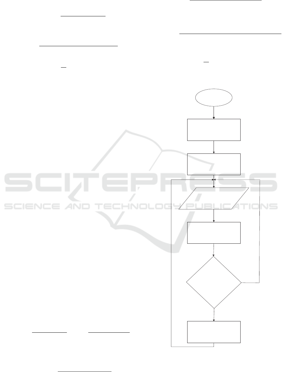
Start

Initialize the

kernel parameters

Learn the ﬁrst

batch using RHPNN

Sequential

introduction

of data

Updating kernel

parameters using

(14)-(19)

Was the

pattern

classiﬁed

correctly?

Add a new kernel

at the location of

the pattern

Yes

Figure 1: Flow chart of the SHPNN algorithm.

It evident that by storing the previous sum of weights

in the memory, we have eliminated the need to have the

entire training sample in each training step. It is also

A Sequential Heteroscedastic Probabilistic Neural Network for Online Classiﬁcation

451

Table 1: Speciﬁcation of datasets used to evaluate SHPNN.

Dataset # Attributes # Classes # Training data # Testing data

iris 4 3 120 30

Image segmentation 19 7 2100 210

Satellite image 36 7 4435 2000

Table 2: Comparison between the performance of SHPNN and other prominent online supervised learning algorithms in

different datasets.

Dataset Algorithm Training time (s) Training accuracy Testing accuracy # Nodes

iris

SNN - 0.872 0.861 -

SHPNN 0.1829 0.9617 0.9267 13.5

Image segmentation

OS-ELM (RBF) 9.9981 0.9700 0.9488 180

SAO-ELM 9.1644 0.9725 0.9516 191

MRAN 7004.5 - 0.9330 53.1

SHPNN 4.4922 0.9426 0.9495 178.3

Satellite Image

OS-ELM (RBF) 319.14 0.9318 0.8901 400

SAO-ELM 211.034 0.9480 0.9139 413

MRAN 2469.4 - 0.8636 20.4

SHPNN 26.44 0.8867 0.8575 534.6

worth noting that since the Jack-knife cannot be used

without having the whole dataset available, it has been

replaced by a simple threshold for variance to avoid nu-

merical difﬁculties when facing sparse data.

If after updating the network parameters in the k+1-

th step the k+1-th pattern is not classiﬁed correctly, then

a new node centered at the pattern in question will be

added to the appropriate kernel group. The variance of

this kernel is set at a small value (about 0.01). In addi-

tion, the existing βs will be scaled so that with the addi-

tion of the new node their sum would stay at one. This

process is summerized in Fig. 1.

4 RESULTS

In order to evaluate the performance of the proposed al-

gorithm, three standard benchmarks were used. These

benchmarks are iris, image segmentation, and satellite

image datasets all from UCI machine learning reposi-

tory (Dua and Graff, 2017). The setup for these tests was

equipped with an Intel Core i7-8550U at 4 GHz with 8

GB of RAM. The speciﬁcations of these datasets are pre-

sented in TABLE 1.

The ﬁrst dataset is Fisher’s Iris dataset that contains

the measured values of sepal and petal dimensions for

three types of Iris plant. The dataset contains 50 patterns

for each type.

The second dataset is image segmentation that con-

sists of a database of images that were drawn arbitrary

from 7 outdoor images and contains 2310 regions of 3x3

pixels. The aim here is to recognize which category

each of these regions belong. These categories consist

of brick facing, foliage, cement, sky, window, grass, and

path. From each of these regions 19 attributes were ex-

tracted.

The ﬁnal dataset used for performance evaluation

of this algorithm is satellite image. It consists of a

databased derived from Landsat multispectral scanner.

Each frame of this scanner imagery comprises of four

digital images of a scene in four different spectral bands.

This dataset is a part of a scene with the size of 82x100

pixels and each pattern in the dataset is a region of 3x3

pixels. The goal here is to classify the central pixel in

a region into 7 categories of red soil, cotton crop, grey

soil, damp gray soil, soil with vegetation stubble, mix-

ture class, and very damp gray soil. It is worth noting

that there are no patterns belonging to the sixth class and

the dataset effectively has 6 classes.

In each dataset, the members of training and test sets

are constant, but the order of their introduction to the

algorithm is shufﬂed in each run.

For each test, the algorithm starts with three kernels

in each group for iris and ﬁve kernels in each group for

the other two datasets. In addition, 10 percent of the

training data is used as the initial batch. For each dataset,

the results are averaged over 10 runs and they are com-

pared with some of the prominent online supervised al-

gorithms in the literature. The results of the tests is pre-

sented in TABLE 2.

It is evident that the proposed algorithm can achieve

good accuracy when comparing with other prominent

online supervised learning algorithms. The training time

for each dataset is also among the best in the litera-

ture. However, the training times for other algorithms

are taken from the respective papers reporting their re-

sults and for a fair comparison, all of the algorithms

should be tested on the same setup.

It is worth noting that the closest algorithm in terms

NCTA 2019 - 11th International Conference on Neural Computation Theory and Applications

452

of both structure and performance to the SHPNN is

SAO-ELM. In the presented algorithm, the initial num-

ber of hidden layer nodes is 35 in the image segmen-

tation and satellite image datasets and this number rose

to 178.3 and 534.6 automatically. On the other hand,

the initial number of hidden nodes for SAO-ELM is 180

and 400 for these datasets respectively, which are opti-

mal node numbers for OS-ELM, and these numbers rose

to 191 and 413. In other words, it appears that the initial

number of nodes for SAO-ELM needs to be very close to

the optimal value, but the SHPNN is capable of ﬁnding

its optimal structure from a very rudimentary initial con-

ﬁguration. This property makes SHPNN a well-suited

algorithm to simulate anthropomorphic learning process.

One of the important properties of the proposed al-

gorithm (which also applies to RHPNN) is the fact that

its hidden node kernels can be used to determine sub-

categories in data and can be used to get a sense of the

statistics of the classes. This property of SHPNN is in

line with the recent trend in machine learning commu-

nity to design interpretable algorithms.

5 CONCLUSIONS

In this paper, a novel algorithm for online supervised

classiﬁcation is presented and its performance is com-

pared with other similar algorithms. The results show

that this algorithm has a great potential in terms of both

speed and accuracy. It is also worth noting that the al-

gorithm is still at the development phase and as future

work, more formula are developed to change the vari-

ances and centers adaptively, while the linking weights

can be adjusted too.

REFERENCES

Asgary, R., Mohammadi, K., and Zwolinski, M. (2007).

Using neural networks as a fault detection mecha-

nism in mems devices. Microelectronics Reliability,

47(1):142–149.

de Jes

us Rubio, J. (2017). A method with neural networks

for the classiﬁcation of fruits and vegetables. Soft

Computing, 21(23):7207–7220.

Dua, D. and Graff, C. (2017). UCI machine learning repos-

itory.

Giap, C. N., Son, L. H., and Chiclana, F. (2018). Dynamic

structural neural network. Journal of Intelligent &

Fuzzy Systems, 34(4):2479–2490.

Hamid, O. H. and Braun, J. (2017). Reinforcement learn-

ing and attractor neural network models of associative

learning. In International Joint Conference on Com-

putational Intelligence, pages 327–349. Springer.

Huang, G.-B., Saratchandran, P., and Sundararajan, N.

(2004). An efﬁcient sequential learning algorithm for

growing and pruning rbf (gap-rbf) networks. IEEE

Transactions on Systems, Man, and Cybernetics, Part

B (Cybernetics), 34(6):2284–2292.

LeCun, Y. A., Bottou, L., Orr, G. B., and M

uller, K.-

R. (2012). Efﬁcient backprop. In Neural networks:

Tricks of the trade, pages 9–48. Springer.

Li, G., Liu, M., and Dong, M. (2010). A new online learn-

ing algorithm for structure-adjustable extreme learn-

ing machine. Computers & Mathematics with Appli-

cations, 60(3):377–389.

Liang, N.-Y., Huang, G.-B., Saratchandran, P., and Sun-

dararajan, N. (2006). A fast and accurate online se-

quential learning algorithm for feedforward networks.

IEEE Transactions on neural networks, 17(6):1411–

1423.

Platt, J. (1991). A resource-allocating network for function

interpolation. MIT Press.

Somu, N., MR, G. R., Kalpana, V., Kirthivasan, K., and

VS, S. S. (2018). An improved robust heteroscedastic

probabilistic neural network based trust prediction ap-

proach for cloud service selection. Neural Networks,

108:339–354.

Venkatesan, R. and Er, M. J. (2016). A novel progressive

learning technique for multi-class classiﬁcation. Neu-

rocomputing, 207:310–321.

Wang, J., Belatreche, A., Maguire, L., and Mcginnity, T. M.

(2014). An online supervised learning method for

spiking neural networks with adaptive structure. Neu-

rocomputing, 144:526–536.

Yang, Z. R. and Chen, S. (1998). Robust maximum like-

lihood training of heteroscedastic probabilistic neural

networks. Neural Networks, 11(4):739–747.

Yang, Z. R., Zwolinski, M., Chalk, C. D., and Williams,

A. C. (2000). Applying a robust heteroscedastic prob-

abilistic neural network to analog fault detection and

classiﬁcation. IEEE Transactions on computer-aided

design of integrated circuits and systems, 19(1):142–

151.

Yingwei, L., Sundararajan, N., and Saratchandran, P.

(1997). A sequential learning scheme for function ap-

proximation using minimal radial basis function neu-

ral networks. Neural computation, 9(2):461–478.

A Sequential Heteroscedastic Probabilistic Neural Network for Online Classiﬁcation

453