VISUAL SERVOING TECHNIQUES FOR CONTINUOUS

NAVIGATION OF A MOBILE ROBOT

N. Garc

ıa, O. Reinoso, J.M. Azor

ın

Dept. Ingenier

ıa de Sistemas Industriales. Universidad Miguel Hern

andez.

Avd. de la Universidad s/n. Edif. Torreblanca. 03202 Elche, Spain

E. Malis

Institut National de Recherche en Informatique et Automatique

2004, route des Lucioles - B.P. 93, 06902 Sophia Antipolis Cedex, France.

R. Aracil

Departamento de Automtica, Electrnica e Informtica Industrial Universidad Politcnica de Madrid.

ETSII c/ Jos Gutirrez Abascal, 2 E-28006 Madrid, Spain.

Keywords:

Visual servoing, mobile robots, navigation, control.

Abstract:

A new method to control the navigation of a mobile robot which is based on visual servoing techniques is

presented. The new contribution of this paper could be divided in two aspects: the ﬁrst one is the solution

of the problem which takes place in the control law when features appear or disappear from the image plane

during the navigation; and the second one is the way of providing to the control system the reference path that

must be followed by the mobile robot. The visual servoing techniques used to carry out the navigation are the

image-based and the intrinsic-free approaches. Both are independent of calibration errors which is very useful

since it is so difﬁcult to get a good calibration in this kind of systems. Also, the second technique allows us to

control the camera in spite of the variation of its intrinsic parameters. So, it is possible to modify the zoom of

the camera, for instance to get more details, and drive the camera to its reference position at the same time. An

exhaustive number of experiments using virtual reality worlds to simulate a typical indoor environment have

been carried out.

1 INTRODUCTION

The framework for robot navigation is based on pre-

recorded image features obtained during a training

walk. Then, we want that the mobile robot repeat

the same walk by means of image-based and invari-

ant visual servoing techniques in a continuous way.

In this point, the question is what does a continuous

way mean?. Well, the answer to this question will be

developed in the following sections of the paper but

in advance the concept continuous way is referred to

assure the continuity of the control law with the ap-

pearance/disappearance of image features during the

control task.

There are some references about using pre-

recorded images to control the navigation of a mobile

robot but all of these applications use them in a dif-

ferent way. For instance, in (Matsumoto et al., 1996)

the control system proposed for the navigation of a

mobile robot is based on a visual representation of

the route called ”View-Sequenced Route Representa-

tion(VSRR)”. After the VSRR was acquired, the robot

repeat the walk using an appearance-based method to

control it by comparing the current view with pre-

recorded one (VSRR).

There are some applications using visual servo-

ing techniques for navigation of a mobile robot. In

(R. Swain-Oropeza, 1997), the application of a visual

servoing approach to a mobile robot which must ex-

ecute coordinate motions in a known indoor environ-

ment is presented. The main contribution of this paper

was the execution of a path expressed as sequence of

several basic motions(like Go to an object, Follow a

wall, Turn around a corner,...):each one is a visually-

guide movement. In our case, the approximation pro-

posed to the navigation is totally different in the way

of dealing with the features which go in/out of the

image plane during the path and similar to some ref-

erences, commented above, in the way of specifying

the path to be followed by the robot.

2 AUTONOMOUS NAVIGATION

USING VISUAL SERVOING

TECHNIQUES

The key idea of this method is to divide the au-

tonomous navigation in two stages: the ﬁrst one is the

training step and the second one is the autonomous

343

García N., Reinoso O., M. Azorín J., Malis E. and Aracil R. (2004).

VISUAL SERVOING TECHNIQUES FOR CONTINUOUS NAVIGATION OF A MOBILE ROBOT.

In Proceedings of the First International Conference on Informatics in Control, Automation and Robotics, pages 343-348

DOI: 10.5220/0001134903430348

 SciTePress

navigation step. During the training step, the robot is

human commanded via radio link or whatever inter-

face and every sample time the robot acquires an im-

age, computes the features and stores them in mem-

ory. Then, from near its initial position, the robot re-

peat the same walk using the reference features ac-

quired during the training step. The current features

and a visual servoing approach is used to minimize

the error between current and reference features.

2.1 Control law

To carry out the autonomous navigation of robot, the

image-based and invariant visual servoing approaches

was used (Hutchinson et al., 1996)(Malis and Cipolla,

2000). Both approaches are based on the selection of

a set s of visual features or a set q of invariant features

that has to reach a desired value s

∗

or q

∗

. Usually, s is

composed of the image coordinates of several points

belonging to the considered target and q is computed

as the projection of s in the invariant space calculated

previously. In the case of our navigation method, s

∗

or q

∗

is variable with time since in each sample time

the reference features is updated with the desired tra-

jectory of s or q stored in the robot memory in order

to indicate the path to be followed by the robot.

To simplify in this section, the formulation pre-

sented is only referred to image-based visual servo-

ing. All the formulation of this section can be applied

directly to the invariant visual servoing approach

changing s by q. The visual task function(Samson

et al., 1991) is deﬁned as the regulation of an error

function:

e = C(s − s

∗

(t)) (1)

The derivative of the task function,considering C con-

stant, will be:

˙e = CLv − C ˙s

∗

(2)

where v = (V

, ω

) is the camera velocity screw

and L is the interaction matrix.

A simple control law can be obtained by imposing

the exponential convergence of the task function to

zero:

˙e = −λ e so CLv = −λ e + C ˙s

∗

(3)

where λ is a positive scalar factor which tunes the

speed of convergence:

v = −λ (CL)

−1

e + (CL)

−1

C ˙s

∗

(4)

if C is setting to L

, then (CL) > 0 and the task

function converge to zero and, in the absence of local

minima and singularities, so does the error s − s

∗

. Fi-

nally substituting C by L

in equation (8), we obtain

the expression of the camera velocity that is sent to

the robot controller:

v = −λ L

(s − s

∗

(t)) + L

˙s

∗

(5)

3 DISCONTINUITIES IN VISUAL

NAVIGATION

In this section, we describe more in details the discon-

tinuity problem that occurs when some features go

in/out of the image during the vision-based control.

The navigation of a mobile robot is a typical example

where this kind of problems are produced.

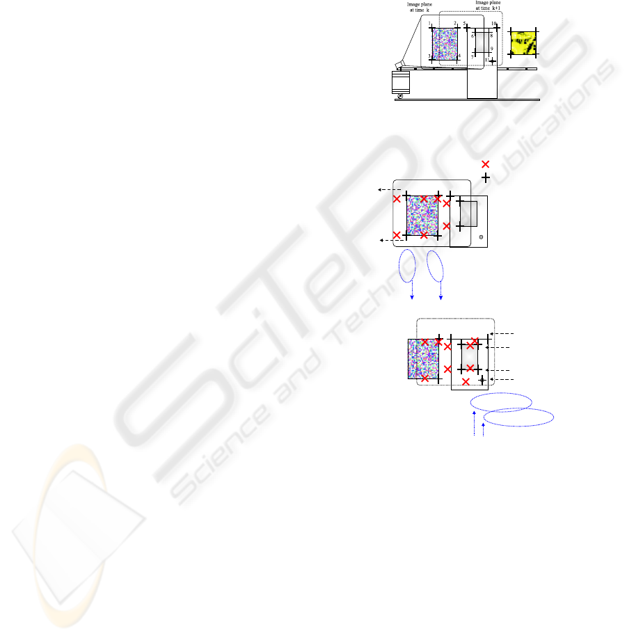
(a) Croquis of the au-

tonomous navigation of the

robot

1 2

Image plane at time k

Image plane at time k+1

at time k+1

Reference features

Current features

s = ( , s , , s , s , s ,s )s s

1 32 4 5 6 7

s = ( , )

* T

s , , s , s , s , s

* * * * *

2 4 5 6 7

Remove

s = ( s , s , s , s , s )

2 4 5 6 7

, s , s , s , s

8 9 10 11

Add

s = ( s , s , s , s , s , )

* * * * * * T

2 4 5 6 7

s , s , s , s

* * * *

8 9 10 11

(b) Appearance/Disappearance of

image features from time k to k+1

Figure 1: Navigation of a mobile robot controlled by visual

servoing techniques.

During autonomous navigation of the robot, some

features appear or disappear from the image plane so

they will must be added to or removed from the visual

error vector (Figure 1). This change in the error vec-

tor produces a jump discontinuity in the control law.

The magnitude of the discontinuity in control law de-

pends on the number of the features that go in or go

out of the image plane at the same time, the distance

between the current and reference features, and the

pseudoinverse of interaction matrix.

In the case of using the invariant visual servoing ap-

proach to control the robot, the effect produced by the

ICINCO 2004 - ROBOTICS AND AUTOMATION

344

appearance/disappearance of features could be more

important since the invariant space Q used to compute

the current and the reference invariant points(q, q

∗

)

changes with features(Malis, 2002c).

4 CONTINUOUS CONTROL LAW

FOR NAVIGATION

In the previous section, the continuity problem of the

control law due to the appearance/disappearance of

features has been shown. In this section a solution

based on weighted features is presented.

4.1 Weighted features

The question is What is a weighted feature?. The an-

swer is obvious it’s a feature which is pre-multiplied

by a factor called weight. This weight is going to be

used in order to anticipate in some way the possible

discontinuities produced in the control law by the ap-

pearance/disappearance of the image features.

The key idea in this formulation is that every fea-

ture (points, lines, moments, etc) has its own weight

which may be a function of image coordinates(u,v)

and/or a function of the distance between feature

points and an object which would be able to occlude

them, etc. In this paper the weights are computed by

a function that depends on the position of image fea-

ture(u,v). Representing the weight as γ

, the function

that has been used and tested to compute the magni-

tude of the weights is:

(x) =







−

(x−x

med

)

(x−x

min

)

max

−x)

min

< x < x

max

0 x = {x

min

, x

max

}

The function weight γ

(x) is a bell-shaped func-

tion which is symmetrical respect to x

med

min

max

.With n, m parameters, the shape of the

bell function can be controlled. Their values must be

chosen according to the following conditions:







min

+ β(x

max

− x

min

)) ≥ 1 − α

min

max

− x

min

)) ≤ α

where 0 < α < 0.5 and 0 < β < 0.5. if the condi-

tions (6)are veriﬁed then the following conditions are

truth too:







max

− β(x

max

− x

min

)) ≥ 1 − α

max

−

max

− x

min

)) ≤ α

where 0 < α < 0.5 and 0 < β < 0.5. For each

feature with (u

, v

) coordinates, a weight γ

(x) for

its u

and v

coordinates can be calculated using the

deﬁnition of the function γ

(x) (γ

= γ

) and

= γ

) respectively). Finally, for every image

feature, a total weight that will be denoted (γ

) is

computed by multiplying the weight of its u coordi-

nate (γ

) by the weight of its v coordinate (γ

4.2 Smooth Task function

Suppose that n matched points are available in the

current image and in the reference features stored.

Everyone of these points(current and reference) will

have a weight γ

which can be computed as it’s

shown in the previous subsection 4.1. With them and

their weights, a task function can be built (Samson

et al., 1991):

e = CW (s − s

∗

(t)) (6)

where W is a (2n × 2n) diagonal matrix where its

elements are the weights γ

of the current features

multiplied by the weights of the reference features.

The derivate of the task function,considering C

constant, will be:

˙e = CW Lv − CW˙s

∗

+ C

W (s − s

∗

) (7)

A simple control law can be obtained by imposing the

exponential convergence of the task function to zero

(˙e = −λ e):

CWLv − CW˙s

∗

+ C

W(s − s

∗

) = −λe (8)

Let us suppose that these weights γ

are varying

slowly, then

W can be considered nearly equal to

zero (

W ≈ 0). Considering this assumption, the

equation (8) can be rewritten as:

v = −λ (CWL)

−1

e + (CWL)

−1

CW˙s

∗

(9)

Setting C = (WL)

, if (CWL) > 0 then the task

function converges to zero and, in the absence of local

minima and singularities, so does the error s − s

∗

Finally substituting C by (WL)

in equation (9), we

obtain the expression of the camera velocity that is

sent to the robot controller:

v = −λ (WL)

W(s−s

∗

(t))+(WL)

W˙s

∗

(10)

4.3 Invariant visual servoing with

weighted features

The theoretical background about invariant vi-

sual servoing can be extensively found in (Malis,

2002b)(Malis, 2002c). In this section, we modify the

approach in order to take into account weighted fea-

tures. Suppose that n image points are available. The

weights γ

used in the weighted invariant visual ser-

voing are obtained as follows:

i=1

(γ

)

· γ

(11)

The weights γ

deﬁned in the previous subsection

are redistributed in order to have

= n. Ev-

ery image point with projective coordinates p

VISUAL SERVOING TECHNIQUES FOR CONTINUOUS NAVIGATION OF A MOBILE ROBOT

345

, v

, 1) is multiplied by its own weight γ

in or-

der to obtain a weighted point p

= γ

. Using

all the weighted points we can compute the following

symmetric (3×3) matrix:

i=1

(12)

The image points depends on the upper triangular ma-

trix K containing the camera intrinsic parameter and

on the normalized image coordinates m

: p

= Km

Thus, we have p

= K(γ

) = Km

and the ma-

trix S

can be written as follows:

i=1

= K S

(13)

where S

is a symmetric matrix which is does not di-

rectly depend on the camera parameters. If the points

are not collinear and n > 3 then S

and S

are posi-

tive deﬁnite matrices and they can be written, using a

Cholesky decomposition, as:

= T

and S

= T

(14)

From equations (13) and (14), the two transformation

matrices, can be related by:

= K T

(15)

The matrix T

deﬁnes a projective transformation

and can be used to deﬁne a point in a new projective

space Q

= T

−1

= T

−1

= T

−1

(16)

The new projective space Q

does not depend di-

rectly on camera intrinsic parameters but it only de-

pends on the weights γ

and on the normalized points.

The normalized points m

depends on a (6×1) vec-

tor ξ containing global coordinates of an open subset

subset S ⊂ R

× SO(3) (i.e. represents the posi-

tion of the camera in the Cartesian space). Suppose

that a reference image of the scene, corresponding to

the reference position ξ

∗

has been stored and com-

puted the reference points p

∗

in a previous learning

step. The camera parameters K

∗

are eventually dif-

ferent from the current camera parameters. We use

the same weights γ

to compute the weighted refer-

ence p

∗γ

= γ

∗

. Similarly to the current image, we

can deﬁne a reference projective space:

∗

= T

∗

−1

∗

= T

∗

−1

∗

(17)

Note that, since the weights in equations (16) and (17)

are the same, if ξ = ξ

∗

then q

= q

∗

∀ i ∈ {1, . . . , n}

and the converse is true even if the intrinsic parame-

ters change during the servoing.

4.3.1 Control in the weighted invariant space

Similarly to the standard invariant visual servoing,

the control of the camera is achieved by stacking

all the reference points of space Q

in a (3n×1)

vector s

∗

(ξ

∗

) = (q

∗

(t), q

∗

(t), · · · , q

∗

(t)). Sim-

ilarly, the points measured in the current camera

frame are stacked in the (3n×1) vector s(ξ) =

(t), q

(t), · · · , q

(t)). If s(ξ) = s

∗

(ξ

∗

) then

ξ = ξ

∗

and the camera is back to the reference po-

sition whatever the camera intrinsic parameters. The

derivative of vector s is:

s = L v (18)

where the (3n×6) matrix L is called the interac-

tion matrix and v is the velocity of the camera.

The interaction matrix depends on current normal-

ized points m

(ξ) ∈ M (m

can be computed from

image points m

= K

−1

), on the invariant

points q

(ξ) ∈ Q

, on the current depth distribu-

tion z(ξ) = (Z

, Z

, ..., Z

) and on the current re-

distributed weights γ

. The interaction matrix in the

weighted invariant space (L

= T

−C

))is

obtained like in (Malis, 2002a) but the term C

must be recomputed in order to take into account the

redistributed weights γ

In order to control the movement of the camera,

we use the control law (10) where W depends on the

weights previously deﬁned and L is the interaction

matrix recomputed for the invariant visual servoing

with weighted features.

5 EXPERIMENTS IN A VIRTUAL

INDOOR ENVIRONMENT

Exhaustive experiments have been carried out using

a virtual reality tool for modelling an indoor envi-

ronment. To make more realistic simulation, errors

in intrinsic and extrinsic parameters of the camera

mounted in the robot have been considered. An es-

timation

K of the real matrix K has been used with

an error of 25% in focal length and a deviation of

50 pixels in the position of the optical center. Also

an estimation

of the camera pose respect to the

robot frame has been computed with a rotation er-

ror of uθ = [3.75 3.75 3.75]

degrees and transla-

tion error of t = [2 2 0]

cm. We are only going

to present the results of one experiment where image

based and invariant visual servoing and the new for-

mulation with weighted features are used to control

the autonomous navigation of an holonomic mobile

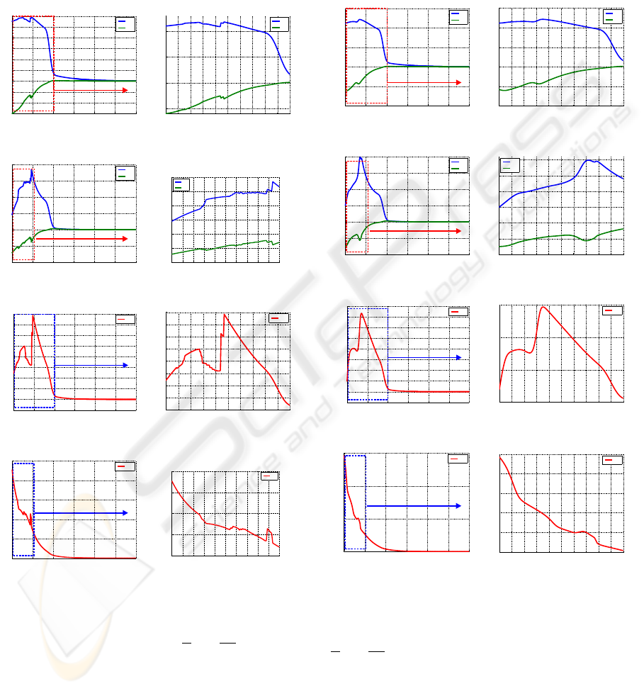
robot. In Figure 3, the control signals sent to the robot

controller using the image-based and invariant visual

servoing approaches are shown. In Figure 3 (b,d,f,h),

ICINCO 2004 - ROBOTICS AND AUTOMATION

346

details of the control law, where the discontinuities

can be clearly appreciated, are presented. To show

the improvements of the new formulation presented in

this paper, the control law using the image-based and

invariant visual servoing with weighted features can

be seen in Figure 4. The same details of the control

law shown in Figure 3 (b,d,f,h) are presented in Fig-

ure 4 (b,d,f,h). Observing both ﬁgures, the improve-

ments respect to the continuity of the control law are

self-evident.

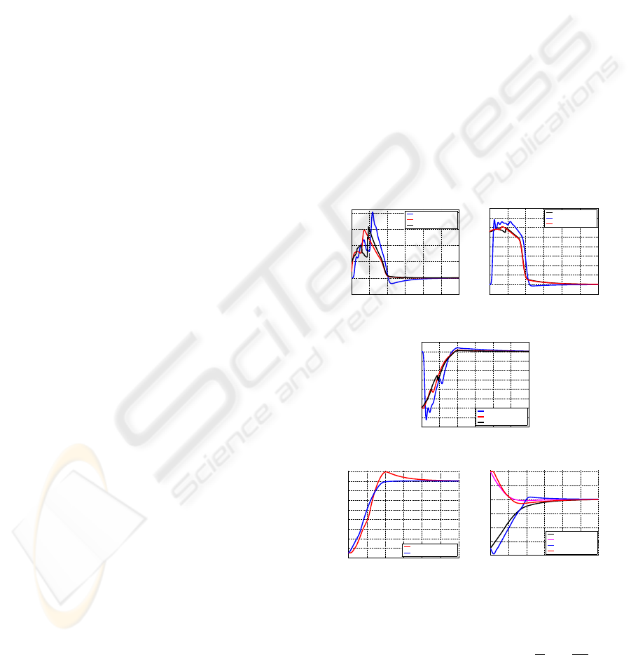
Some experiments using a ﬁlter to avoid the effects

of the discontinuities in the control law have been car-

ried out too. A 8th order butterworth lowpass digi-

tal ﬁlter has been designed to overpass the disconti-

nuities produced by the appearance/disappearance of

image features. In Figure 2 (a,b,c), the continuity of

the control law using a ﬁlter or weighted features and

the discontinuity with the classical image-based ap-

proach can be seen. However the trajectory of the

mobile robot is not the same using weighted features

than ﬁltering the control law (Figure 2 (d,e)). Fur-

thermore the trajectory error when the control law is

ﬁltered needs more time to stabilize than when the

formulation with weighted features is used.

6 CONCLUSION

In this paper the originally formulation of two visual

servoing approaches, which avoids the discontinuities

in the control law when features go in/out of the im-

age plane during the control task, is presented and

tested by several experiments in a virtual indoor en-

vironment. The results presented corroborate that the

new approach to the problem works better than a sim-

ple ﬁlter of the control signals. The validation of this

results with a real robot is on the way by using a

B21r mobile robot from iRobot company. As a fu-

ture work, it would be interesting to test another kind

of weighted functions.

REFERENCES

Hutchinson, S. A., Hager, G. D., and Corke, P. I. (1996). A

tutorial on visual servo control. IEEE Trans. Robotics

and Automation, 12(5):651–670.

Malis, E. (2002a). Stability analysis of invariant visual

servoing and robustness to parametric uncertainties.

In Second Joint CSS/RAS International Workshop on

Control Problems in Robotics and Automation, Las

Vegas, Nevada.

Malis, E. (2002b). A uniﬁed approach to model-based

and model-free visual servoing. In European Confer-

ence on Computer Vision, volume 2, pages 433–447,

Copenhagen, Denmark.

Malis, E. (2002c). Vision-based control invariant to camera

intrinsic parameters: stability analysis and path track-

ing. In IEEE International Conference on Robotics

and Automation, volume 1, pages 217–222, Washing-

ton, USA.

Malis, E. and Cipolla, R. (2000). Self-calibration of zoom-

ing cameras observing an unknown planar structure.

In Int. Conf. on Pattern Recognition, volume 1, pages

85–88, Barcelona, Spain.

Matsumoto, Y., Inaba, M., and Inoue, H. (1996). Vi-

sual navigation using view-sequenced route represen-

tation. In IEEE International Conference on Robotics

and Automation (ICRA’96), volume 1, pages 83–88,

Minneapolis, USA.

R. Swain-Oropeza, M. D. (1997). Visually-guided naviga-

tion of a mobile robot in a structured environment. In

International Symposium on Intelligent Robotic Sys-

tems (SIRS’97), Stockholm, Sweden.

Samson, C., Le Borgne, M., and Espiau, B. (1991). Robot

Control: the Task Function Approach. volume 22 of

Oxford Engineering Science Series.Clarendon Press.,

Oxford, UK, 1st edition.

0 100 200 300 400 500 600

−0.05

0.05

0.1

0.15

0.2

iterations number

Rotation speed

( filter )

( weighted features )

(a)

0 100 200 300 400 500 600

−0.2

0.2

0.4

0.6

0.8

1.2

1.4

1.6

iterations number

Traslational speed V

( filter )

( weighted features )

(b)

0 100 200 300 400 500 600

−0.8

−0.7

−0.6

−0.5

−0.4

−0.3

−0.2

−0.1

0.1

( filter )

( weighted features )

Traslational speed V

Iterations number

(c)

0 100 200 300 400 500 600

−8

−7

−6

−5

−4

−3

−2

−1

Iterations number

θ ( filter )

θ ( weighted features )

(d)

0 100 200 300 400 500 600

−0.8

−0.6

−0.4

−0.2

0.2

0.4

Iterations number

( weighted features )

( filter )

(e)

Figure 2: Image-based visual servoing approach: classical,

with weighted features and using a ﬁlter. The translation

and rotation errors are measured respectively in m and deg,

while speeds are measured respectively in

and

deg

VISUAL SERVOING TECHNIQUES FOR CONTINUOUS NAVIGATION OF A MOBILE ROBOT

347

0 100 200 300 400 500 600

-0.6

-0.4

-0.2

0.2

0.4

0.6

0.8

1.2

Traslation speed

Iterations number

Detail

(a) Image-based

0 20 40 60 80 100 120 140 160 180 200

−0.5

0.5

Traslation speed

Iterations number

(b) Details

0 100 200 300 400 500 600

-1

-0.5

0.5

1.5

Traslation speed

Iterations number

Detail

0 10 20 30 40 50 60 70 80 90 100

−1

−0.5

0.5

1.5

(d) Details

0 100 200 300 400 500 600

-0.02

0.02

0.04

0.06

0.08

0.1

0.12

0.14

0.16

Rotation speed

Iterations number

Detail

(e) Image-based

0 20 40 60 80 100 120 140 160 180 200

0.02

0.04

0.06

0.08

0.1

0.12

0.14

0.16

Rotation speed

Iterations number

(f) Details

0 100 200 300 400 500 600

0.05

0.1

0.15

0.2

0.25

Rotation speed

Iterations number

Detail

(g) Invariant

0 10 20 30 40 50 60 70 80 90 100

0.05

0.1

0.15

0.2

0.25

(h) Details

Figure 3: Control law: Image-based(a,b,e,f) and invari-

ant(c,d,g,h) visual servoing. The translation and rotation

speeds are measured respectively in

and

deg

0 100 200 300 400 500 600

-1

-0.5

0.5

1.5

Traslation speed

Iterations number

Detail

(a) Image-based

0 20 40 60 80 100 120 140 160 180 200

−1

−0.5

0.5

1.5

Traslation speed

Iterations number

(b) Details

0 100 200 300 400 500 600

-1

-0.5

0.5

1.5

Traslation speed

Iterations number

Detail

0 10 20 30 40 50 60 70 80 90 100

−1

−0.5

0.5

1.5

Traslation speed

Iterations number

(d) Details

0 100 200 300 400 500 600

-0.02

0.02

0.04

0.06

0.08

0.1

0.12

0.14

0.16

Rotation speed

Iterations number

Detail

(e) Image-based

0 20 40 60 80 100 120 140 160 180 200

0.05

0.1

0.15

Rotation speed

Iterations number

(f) Details

0 100 200 300 400 500 600

0.1

0.2

0.3

Rotation speed

Iterations number

Detail

(g) Invariant

0 10 20 30 40 50 60 70 80 90 100

0.05

0.1

0.15

0.2

0.25

0.3

Rotation speed

Iterations number

(h) Details

Figure 4: Control law: Image-based(a,b,e,f) and invari-

ant(c,d,g,h) visual servoing with weighted features. The

translation and rotation speeds are measured respectively in

and

deg

ICINCO 2004 - ROBOTICS AND AUTOMATION

348