HEXAPOD STRUCTURE EVALUATION AS WEB SERVICE

Leonardo Jelenković, Domagoj Jakobović, Leo Budin

Faculty of Electrical Engineering and Computing, University of Zagreb, Croatia

Keywords: Stewart platform, workspace, error analysis, kinematic parameters, forward kinematics, web services

Abstract: This paper describes several methods for evaluation of kinematic parameters of a Stewart platform. One of

those methods is the calculation of workspace area both in numerical and graphical form. The second

method allows us to analyze and estimate inherent mechanism errors that occur due to actuator errors,

elastic and thermal deformations and other error sources. Furthermore, another procedure is presented which

calculates certain kinematic parameters throughout the workspace area of the model and outputs them as

numerical and graphical data. Finally, a forward kinematics algorithm designed for use in real-time

conditions and its adaptation is presented. The described algorithms are implemented and made available as

web services on the project web site (http://hexapod.zemris.fer.hr/).

1 INTRODUCTION

Parallel kinematic manipulators (PKMs) have been

rediscovered in the last decade as microprocessor's

power finally satisfies computing force required for

their control. Their great payload capacity, stiffness

and accuracy characteristic as result of their parallel

structure make them superior to serial manipulators

in many fields.

One of the most accepted PKMs is Stewart

platform based manipulator, also known as hexapod

or Gough platform. Hexapod, originally, consists of

two platforms, one fixed on the floor or ceiling and

one mobile, connected together via six extensible

struts with spherical or other types of joints. That

construction gives mobile platform 6-DOF (degrees

of freedom). Hexapod movement and control is

achieved only through strut lengths changes. One

variation to this structure, also observed here, is

when struts are fixed in length but one of their ends

is placed on a guideway. Control is then obtained

only by moving the joints positioned on guideways.

Although in this model the forces acting on struts are

not just along the axis of the strut, as in the original

design, practically attainable sliding characteristics

of guideways make it a very considerable structure

for manipulators.

One of the qualities we want from a manipulator

is its good kinematics behavior. The kinematic

characteristics have direct impact on manipulability

and working speed of a manipulator. In this paper

we present several methods for calculating various

kinematic parameters of Stewart platform. These

methods can be used to optimize hexapod structure

for better kinematic characteristics or combined with

other procedures were kinematic can be just one

measure in optimization process.

The forward kinematic (Merlet, 1993) of a

parallel manipulator is the problem of finding the

position and orientation of the mobile platform when

the strut lengths are known. This problem has no

known closed form solution for the most general 6-6

form of hexapod manipulator (with six joints on the

base and six on the mobile platform). In this paper

we present a method for numerical solving of

forward kinematics, which is derived from our

previous work where several mathematical

representations of the forward kinematic problem, in

the form of optimization functions, were combined

with various optimization algorithms and adaptation

methods in order to find an efficient procedure that

would allow for precise forward kinematic solving

in real-time conditions.

2 THE INVERSE KINEMATICS

PROBLEM

The inverse kinematics problem compared to

forward kinematics is almost trivial for parallel

manipulator such as hexapod. Inverse kinematics

will be presented here for two different hexapod

492

Jelenkovi

c L., Jakobovi

c D. and Budin L. (2004).

HEXAPOD STRUCTURE EVALUATION AS WEB SERVICE.

In Proceedings of the First International Conference on Informatics in Control, Automation and Robotics, pages 492-497

DOI: 10.5220/0001136504920497

 SciTePress

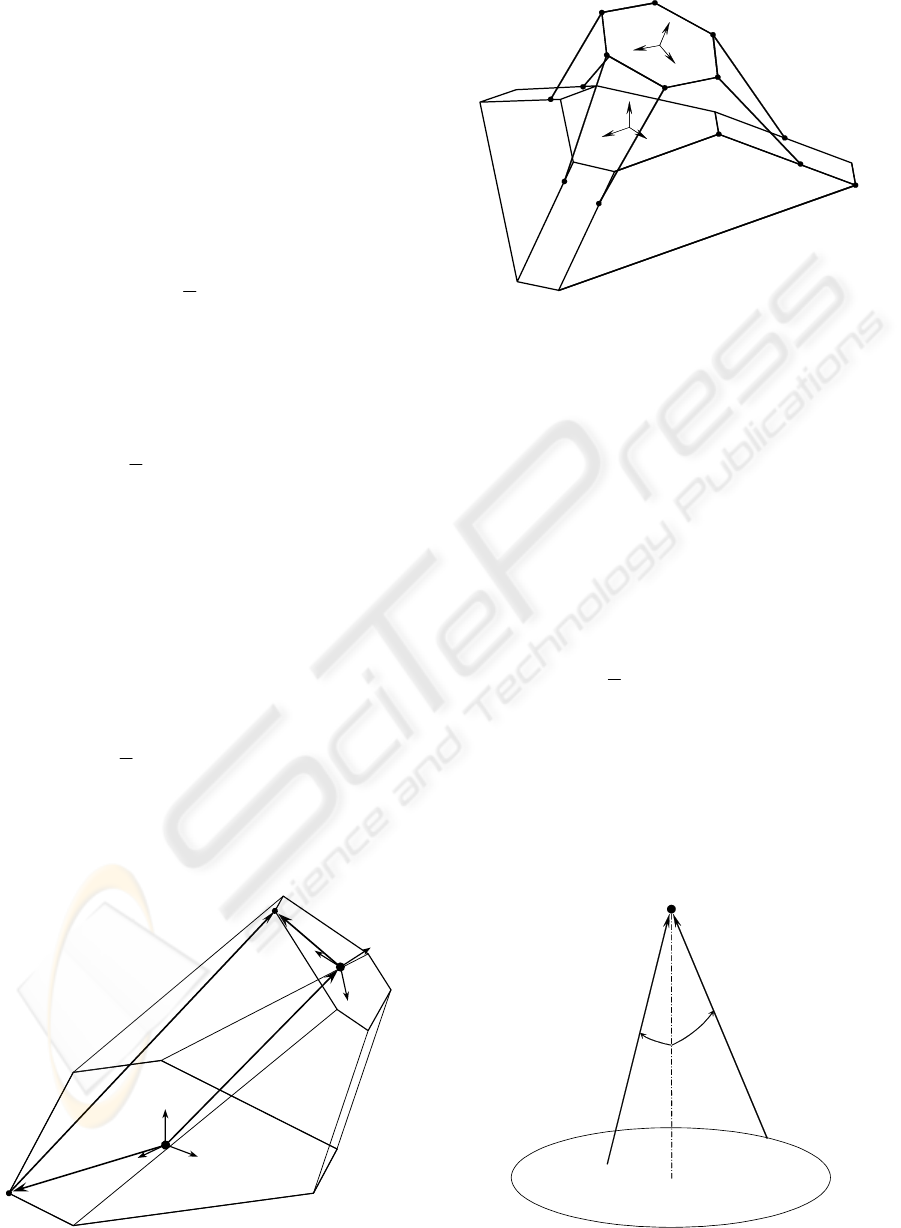
structures: standard Stewart platform based

manipulator as shown in Figure 1 and hexapod

shown on Figure 2.

Standard Stewart Platform based manipulator as

shown in Figure 1 can be defined with: minimal and

maximal struts length (l

min

, l

max

), radii of fixed and

mobile platforms (r

, r

), joint placement defined

with angle between closest joints for both platforms

(

) and joint moving area (assuming cone with

angle

Inverse kinematics can be described with

equations:

()

iii

BAdq

aRrA

⋅+=

(1)

(2)

where

and

are joint position vectors on

base and mobile platform,

are joint position

vectors of mobile platform,

are joint position

vectors in local coordinate system of mobile

platform,

is translation vector between base and

mobile systems,

R is orientation matrix of mobile

platform, d() is distance funtion and

q are strut

lengths calculated with inverse kinematics.

The second observed hexapod model, shown in

Figure 1, differs from standard Stewart manipulator

at base platform and struts. Strut lengths are constant

but their joints on one side are placed on sliding

guide-ways where actuators are placed. Parameters

which describe this model differ only for base

platform:

and

define i

guide way and s

as value between [0, 1] identify actual joint position.

Inverse kinematics for this model can be defined

using equations:

()

,,,

,,, ipikiipi

iii

BBsBB

BAdlaRrA

rrrr

−⋅+=

=⋅+=

(3)

Values s

are calculated from quadratic equation

and therefore can give two possible joint positions

on same guide way. This problem must be solved in

control procedures.

⋅

Figure 1: Stewart Platform manipulator

Figure 2: Hexapod with fixed strut lengths

End effector (tool) is placed on mobile platform

above the geometrical center of joints placed on that

platform by height l

tool

. Therefore, origin of local

coordinate system of mobile platform is placed in

that point. Subsequently vectors

and

are

calculated for that origin.

In our work inverse kinematics is used for

calculating three hexapod characteristics: workspace

volume, error study and kinematics evaluation.

3 WORKSPACE CALCULATION

For given end effector (tool) position and

orientation, defined with translation vector

and

rotation matrix

R , joint positions on mobile

platform

can be calculated. Using inverse

kinematics strut lengths

q and directions

can be

calculated for first model, and joint positions

s and

directions

, for second model. With these values

it is possible to check if hexapod is able to put its

mobile platform to required position verifying

several constraints.

Firstly, strut lengths must be within given ranges

for first model or joints must lay on guide ways for

second model.

max

Figure 3: Orientations used in calculations

HEXAPOD STRUCTURE EVALUATION AS WEB SERVICE

493

Secondly, joint constraints must be met.

Spherical joints are used in modeling and its

restrictions checked.

The third and the last constraints which are

checked are struts collisions. Since struts have some

thickness it is possible that collisions between any

two struts occur. For second hexapod model strut

collisions with base platform are also checked.

If all constraint for given end effector are

satisfied then given position is reachable. With a

fixed end effector orientation a predefined volume

can be checked and workspace with given

orientation found.

Assuming that manipulator is used for

machining free surface items, working area can be

better defined as area were manipulator can work for

(almost) any required orientation. Required

orientations which give optimal surface

characteristics are normals to surface itself. Usually

they can be defined with vectors within a cone with

defined angle as shown in Figure 3. Working area

calculated using this definition gives superior visual

and numeric description of manipulator. For

performance reasons such cone is approximated with

a dozen vectors for each of several different angles

smaller than or equal to

max

. In this way the result

isn’t just twofold, and if point isn’t a part of

workspace, information for which

max

it will

eventually be can still be obtained.

Using the described methods, workspace area for

first and second hexapod model can be calculated.

Detailed description can be found in (Jakobović,

2002).

4 ERROR ANALYSIS

Control of hexapod manipulator is based on inverse

kinematics. However, that was valid only for

models. In reality there must be a feedback through

some kind of sensors that measure actual strut

lengths and end-effector position. Because of

unpredictable environment some hexapod elements

may have values different from nominal. This can be

due to the assembly errors, elastic and thermal

deformations, actuator errors and others error

sources (Wang, 1995). Model that includes all

sources of errors is hardly possible to implement

because of nonlinear dependent error sources and

most of error elements can’t even be calculated or

measured. What is shown in this paper is to give an

approximate value for error at end effector if error

sources are given as approximate values

(tolerances), just quantities, not directions.

From Figure 1, for one vector chain through i

strut, the following equation can be deducted:

iii

aRrwqb

⋅+=⋅+

(4)

Differentiating this equation yields:

iiiii

aRaRrwqwqb

δδδδδδ

⋅+⋅+=⋅+⋅+

(5)

which can be interpreted as relations between

errors in joint positions

δδ

and actuator errors

with errors at end effector position r

and

orientation

. Furthermore, two more error

elements are added to (5), errors in joint centre

position (Patel, 1997), both on mobile and fixed

platform:

()

iiiiii

daRaRr

wqwqcb

rrr

+⋅+⋅+

=⋅+⋅++

δδδ

(6)

Multiplying (6) with

, than replacing

RR ⋅Ω=

δδ

, where Ω

is orientation error vector,

and with simple vector and mathematics

transformations (6) becomes (7).

(

)

()()

iiii

cbwdaRw

wawrq

+⋅−+⋅⋅+

+×⋅Ω+⋅=

δδ

δδδ

(7)

Equation (7) can be generalized and used in

matrix form:

()

ANJ

δδδ

⋅−Λ⋅=Π

⋅+Π⋅=Λ

−

(8)

where

[

]

qqq

621

...

δδδδ

=Λ

(9)

[

]

[

]

zyxzyx

rrrr

ωωωδδδδδδ

=Ω=Π

(10)

()

666

111

⎥

⎦

⎤

⎢

⎣

⎡

⎥

⎦

⎤

⎢

⎣

⎡

waw

rrr

(11)

⎥

⎦

⎤

⎢

⎣

⎡

−⋅

TTTT

wRw

MMOMM

(12)

With formula (8) error in position and

orientation at end effector can be calculated if all

errors are known or at least presumed.

Formulas for the second hexapod model can be

achieved following the same procedure, thus

yielding formulas (13) to (16).

()

BANSJ

BANJS

−⋅−Ψ⋅⋅=Π

+⋅+Π⋅=Ψ⋅

−

δδδ

(13)

Equation (13) is an equivalent for (8) for model

with fixed strut lengths. But exact values for each

error element must be known to calculate errors at

end effector.

ICINCO 2004 - ROBOTICS AND AUTOMATION

494

()

⎥

⎦

⎤

⎢

⎣

⎡

⎥

⎦

⎤

⎢

⎣

⎡

=Ψ

waw

666

111

rrr

(14)

⎥

⎦

⎤

⎢

⎣

⎡

⋅

⎥

⎦

⎤

⎢

⎣

⎡

⋅

MOM

(15)

⎥

⎦

⎤

⎢

⎣

⎡

⋅+

⎥

⎦

⎤

⎢

⎣

⎡

666

111

cwq

(16)

What can be done if errors can be only

approximated with some border values? Using worst

case method and formulas (8) or (13) a maximal

error can be found searching through all possible

input error values. This method is used in analysis.

Because of large search space an approximate

iterative numerical method very similar to

coordinate axis search is used to find global

maximum.

5 KINEMATIC ANALYSIS

For kinematics evaluation, the relation between

actuators speed and end effector speed is required.

Observing one vector chain through i

strut for the

first model, the following equation can be written:

iiii

arwqb

+=⋅+

(17)

Since

is unity vector and

=∂∂ rb

derivation of eq. (17) yields eq. (18), where

and

are linear and angular end effector velocities.

iiiii

avwqwq

×+

×⋅+⋅

(18)

Eq. (18) can be easily transformed in form of eq.

(19) and then finally in matrix form as on eq. (20).

This is a final kinematics equation, where relation

between end effector velocity and actuator velocity -

strut lengths changes, is given.

()

iiii

wawvq

⋅×+⋅=

(19)

()

xJq

waw

rrr

⋅=⇔

⎥

⎦

⎤

⎢

⎣

⎡

⋅

⎥

⎦

⎤

⎢

⎣

⎡

666

111

(20)

For second model shown on Figure 2, for one

vector chain through i

strut, the following equation

can be deducted:

iiiii

arwqlsb

rrr

+=⋅+⋅+

(21)

Derivation of eq. (21) yields eq. (22), and with

little more mathematical operations we get

kinematics equation (23) very similar to first

hexapod model.

iiii

avwqls

×+=×⋅+⋅

ωω

(22)

()

xJxKLsxKsL

waw

rrr

MOM

⋅=⋅⋅=⇒⋅=⋅

⎥

⎦

⎤

⎢

⎣

⎡

⎥

⎦

⎤

⎢

⎣

⎡

⎥

⎦

⎤

⎢

⎣

⎡

⎥

⎦

⎤

⎢

⎣

⎡

⋅

−1

666

111

(23)

As equations (20) and (23) show, relation

between end effector velocities and strut changes is

given by a matrix commonly called jacobian.

Kinematics characteristics must therefore be

extracted from that matrix. Commonly used values

for kinematics evaluation of manipulator are

singular values of jacobian (Stoughton, 1993,

Pittens, 1993, Huang, 1998).

Three parameters based on singular values are

usually used for kinematics evaluation:

condition number:

max

min

minimal singular value:

min

manipulability: |det(

′

−1

J )|=Π

Proposed method used to evaluate manipulator

from a kinematic aspect is to calculate those three

parameters through whole workspace of the

manipulator or just in some part of it. For every

point where calculations are to be performed, those

three parameters are calculated not only for one end

effector orientation but for all orientations as shown

on Figure 3. The value for particular kinematics

parameter is then calculated as average value.

6 FORWARD KINEMATICS

In our work we have combined several mathematical

representations of the forward kinematics problem

with various optimization algorithms. The

algorithms applied in this work were Powell's

method, Hooke-Jeeves', steepest descent search,

Newton-Raphson's (NR) method, NR method with

constant Jacobian and Fletcher-Powell algorithm.

Solving of forward kinematic was simulated in

static and dynamic conditions. The goal was to find

the combination which would yield the best results

considering the convergence, speed and accuracy.

The most promising combinations were tested in

dynamic conditions, where the algorithm had to

track a preset trajectory of the mobile platform with

as small error and as large sampling frequency as

possible. The most successful combination was

Newton-Raphson's algorithm applied to canonical

representaion of the problem, of which more

information can be found in (Jakobović, 2002) and

(Dasgupta, 1994).

In dynamic simulation, the starting hexapod

configuration is known and serves as an initial

solution. During the sampling period

T the algorithm

has to find the new solution, which will become the

initial solution in the next cycle. Several hexapod

HEXAPOD STRUCTURE EVALUATION AS WEB SERVICE

495

movements were defined as time dependant

functions of the position and orientation of mobile

platform. One of those trajectories is defined with

() ()

() ( ) () ( )

()

() ( )

.40,42arctan15

,4cos5

sin30

,8.1sin55,2sin38

cos2.2,

sin2

≤≤−⋅=

⋅+

⎟

⎠

⎞

⎜

⎝

⎛

⋅=

⋅=⋅+=

⎟

⎠

⎞

⎜

⎝

⎛

⋅=

⎟

⎠

⎞

⎜

⎝

⎛

⋅=

ttt

ttttz

ttyttx

ππ

(24)

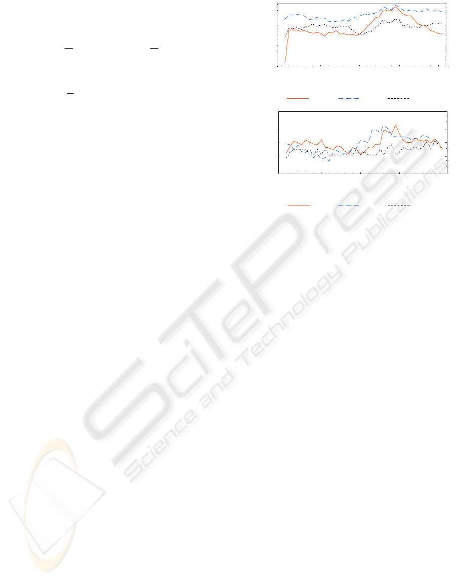
The results of the dynamic simulation are

presented in the form of a graph where errors in the

three rotation angles and three position coordinates

of the mobile are drawn. The sampling period

T was

set to 1 ms, which equals to a 1000 Hz sampling

frequency. The errors shown represent the absolute

difference between the calculated and the actual

hexapod configuration. Due to the large number of

cycles, the error is defined as the biggest absolute

error value in the last 100 ms, so the graphs in each

point show the

worst case in the last 100 ms of

simulation. The errors are presented separately for

angles, in degrees, and position coordinates. The

errors are shown in Figure 3 and Figure 4.

The achieved level of accuracy is very high as

the absolute error does not exceed 10

-12

both for

angles and coordinates.

Mathematical analysis has shown (Raghavan,

1993, Wen, 1994) that there may exist up to 40

distinctive solutions for forward kinematic problem

for Stewart platform with planar base and mobile

platform for the

same set of strut lengths. Let us

suppose that in one hexapod configuration there

exists no other forward kinematic solution for actual

set of strut lengths, but that in some other

configuration there exist several of them. If hexapod

in its movement passes through those two

configurations, then at a certain point in between

there has to be a division point where the number of

solutions increases. In those division points the

solving algorithm may, unfortunately, begin to

follow any of the possible paths, because any of

them represents a valid forward kinematic solution.

If that is the case, the algorithm may either

follow the correct trajectory or the equivalent one. It

is important to note that in both cases the

optimization function remains very low (app. 10

-30

-20

) during the whole process because both

trajectories depict a valid solution. The problem is,

only one of them represents the actual hexapod

configuration in each point of time.

0 10 20

Cycle index

−

Absolute error

Figure 4: Absolute angle error

(

= ,

= )

0 10 20

Cycle index

−

Absolute error

Figure 5: Absolute coordinate error

(

= , y = ,

= )

Without any additional information about the

hexapod configuration, such as may be obtained

from extra transitional displacement sensors, there is

unfortunately no way to determine which of the

existent solutions to the forward kinematic problem

for the same set of strut lengths describes the actual

hexapod configuration. Nevertheless, with some

assumptions we may devise a strategy that should

keep the solving method on the right track. If the

change of the direction of movement is relatively

small during a single period, which is in this case

only 1 ms, then we can try to predict the position of

the mobile platform in the next cycle. We can use

the solutions from the past cycles to construct a

straight line and estimate the initial solution in the

next iteration. Let the solution in the current iteration

and the solutions from the last two cycles

and

. Then we can calculate the new initial

solution using one of the following methods:

100

2 PPX

−⋅= ,

(25)

200

5.05.1 PPX

⋅−⋅=

(26)

(

)

()

⎪

⎭

⎪

⎬

⎫

⋅−⋅=

+⋅=

210

212

101

5.15.2

,5.0

TTX

PPT

rrr

(27)

The above methods were tested for all the

simulated trajectories. The results were very good:

the solving method was able to track the correct

solution during the whole simulation process for all

three estimation methods. The number of conducted

experiments was several hundred and every time the

algorithm's error margin was below 10

-11

both for

angles and coordinates. However, the described

algorithm adaptation will only be successful if the

assumption of a small direction change during a few

ICINCO 2004 - ROBOTICS AND AUTOMATION

496

iterations is valid. To test the algorithm's behavior,

simulated movement was accelerated by factor 2, 4

and 8, while maintaining the same cycle duration of

1 ms. Only by reaching the 8-fold acceleration,

when the total movement time equals a very

unrealistic half a second, did the algorithm produce

more significant errors, while still holding to the

correct solution.

7 HEXAPOD ANALYSIS AS WEB

SERVICE

The described methods of hexapod analysis have

been implemented as Web services at

(http://hexapod.zemris.fer.hr/). Hexapod structure

can be defined through Web interface and then a

particular operation is performed. Workspace

volume can be calculated as a number representing

volume in cubic units, or drawn as VRML shape or

cross-section with horizontal or vertical plane. Error

values and kinematics values can be calculated as

overall values through all workspace or just in cross-

section with a plane.

Implementation is done through CGI programs,

PHP scripting language for Apache Web server,

currently running on a two processor Windows 2000

Server. CGI is chosen because of performance issues

since analysis methods are computationally

intensive. PHP scripts are used to collect hexapod

parameters from users and temporary store them in

session variables. Before calling CGI programs,

PHP script writes parameters to a file on a server.

CGI then reads those files, performs calculations and

produces results. Depending on demanded

calculations, results can be in HTML form, images

or VRML files. VRML format is used for displaying

hexapod models and its workspace. An implicit

surface triangulation method is used for generating

workspace. Improving and optimizing process of

this triangulation method is in progress.

To utilize multiprocessor system a multithreaded

version of program is written since computations can

be easily parallelized. Additional 15-20 percent

speedup is achieved using hyper-threading

technology of Intel Xeon processors.

Regarding speed, workspace calculation can take

up to a few minutes to complete. Kinematics is little

more time demanding, depending on chosen

operation and precision. Error analysis, in spite of

enormous effort in optimizing, is still extremely

slow and time consuming, and it can take 15 to 20

minutes or even more to compute.

8 CONCLUSION

Methods for hexapod analysis are shown, starting

with workspace calculation, error sensitivity analysis

and kinematics evaluation. A forward kinematics

algorithm designed for use in real-time environment

is presented. These methods are prepared and

implemented in a functional Web based system.

ACKNOWLEDGEMENT

This work was carried out within the research

project "Distributed Embedded Computing

Systems", supported by the Ministry of Science and

Technology of the Republic of Croatia.

REFERENCES

Patel, A.J., Ehmann, K.F., 1997. Volumetric Error

Analysis of a Stewart Platform-Based Machine Tool,

Annals of the CIRP, vol. 47/1, pp. 287-290.

Wang, S.M., Ehmann, K.F., 1995. Error Model and

Accuracy Analysis of a Six-DOF Stewart Platform,

Manufacturing Science and Eng., 2-1, pp. 519-530.

Jakobović, D., Jelenković, L., 2002. The Forward and

Inverse Kinematics Problems For Stewart Parallel

Mechanisms,

Int. Sci. Conf. Production Eng.:

CIM2002,

Brijuni, 2002, pp. II-001- II-012.

Huang, T., Whitehouse, D.J., Wang, J., 1998. The Local

Dexterity, Optimal Architecture and Design Criteria of

Parallel Machine Tools,

Annals of the CIRP, vol. 47/1,

pp.347-351.

Stoughton, R.S., Arai, T., 1993. A Modified Stewart

Platform Manipulator with Improved Dexterity,

IEEE

Trans. on Robotics and Automation

, vol. 9, no. 2, pp.

166-173.

Merlet, J.-P., 1993. Direct Kinematic of Parallel

Manipulators,

IEEE Transactions on Robotics and

Automation

, Vol. 9, No. 6, pp. 842-845

Jakobović, D., Budin, L., 2002. Forward Kinematics of a

Stewart Parallel Mechanism,

Proc. 6

Int. Conf. on

Intelligent Engineering Systems INES 2002

, Opatija,

May 26-28., pp.149-154

Dasgupta, B., Mruthyunjaya, T.S., 1994. A Canonical

Formulation of the Direct Position Kinematic Problem

for a General 6-6 Stewart Platform,

Mech. Mach.

Theory

, Vol. 29, No. 6, pp. 819-827,

Raghavan, M., 1993. The Stewart Platform of General

Geometry has 40 Configurations,

Journal of

Mechanical Design

, Vol. 115, pp. 277-282

Wen, F., Liang, C., 1994. Displacement Analysis of the 6-

6 Stewart Platform Mechanisms,

Mechanism and

Machine Theory

, Vol. 29, No. 4, pp. 547-557

HEXAPOD STRUCTURE EVALUATION AS WEB SERVICE

497