ON THE RECONSTRUCTION PERFORMANCE OF
COMPRESSED ORTHOGONAL MOMENTS
G.A.Papakostas, Y.S.Boutalis
Democritus University of Thrace, Department of Electrical and Computer Engineering, 67100 Xanthi, Greece
D.A.Karras
Hellenic Aerospace Industry and University of Hertfordshire, Rodu 2, Ano Iliupolis,16342 Athens, Greece
B.G.Mertzios
Thessaloniki Institute of Technology, Department of Automation, Laboratory of Control Systems and Comp.Intelligence
Keywords: Zernike, Pseudo-Zernike, Fourier-Mellin, orthogonal moments, wavelet compression, image reconstruction
Abstract: In this paper, a wavelet-based technique is applied to three moment featu
re vectors corresponding to three
different families of orthogonal moments. The resulted compressed vectors are studied experimentally, in
order to extract useful information about their behaviour to a reconstruction procedure. The reconstruction
performance of these moments is identical to the amount of image information that they contain to certain
moment orders. Since the moment vectors are imposed to compression at the high frequency components, a
conclusion about their information redundancy can be also determined. The most efficient moment family,
by means of the reconstruction error, will form feature vectors with low dimension, yet with high
information content and thus will be very useful for pattern recognition applications, guarantying high
recognition rates.
1 INTRODUCTION
Image moments have played a major role in vision
systems, since their first introduction by Hu (Hu,
1962). They have been used as image descriptors,
able to characterize an image uniquely. The
uniqueness property unfortunately is satisfied only
by the orthogonal moments, which derived from
orthogonal polynomials consisting an orthonormal
basis. This feature makes them more useful than the
conventional ones, since they guarantee a small
information redundancy and high reconstruction
capabilities.
In general an infinite number of moments can
describe the whole image, but in practical
applications a finite number of them is mostly
needed. Thus, there is a need to use the appropriate
moment feature vector that encloses as much as
possible image information. By applying a
compression method to the moment feature vector,
this requirement is satisfied (Papakostas, 2002,
2004).
In this paper, an investigation about the
reco
nstruction performance of three popular families
of orthogonal moments, which have been processed
by using the above procedure, is attempted. The
present study is focused on the reconstruction
capability of the three compressed moment vectors;
in order to decide which
orthogonal moment family
behaves appropriately, by means of the image
reconstruction error.
The most efficient moment family, which will be
o
btained, can be used in any pattern recognition
task, as a discriminative feature vector, as it has
already been presented in (Papakostas, 2004).
The following sections, are introducing the
Zerni
ke moments (ZMs), Pseudo-Zernike moments
(PZMs) and Fourier-Mellin orthogonal moments
(OFMMs), and the processing algorithm that these
moments will be imposed to. Finally, in the last
section, an experimental study is taking place in
468
A. Papakostas G., S. Boutalis Y., A. Karras D. and G. Mertzios B. (2004).
ON THE RECONSTRUCTION PERFORMANCE OF COMPRESSED ORTHOGONAL MOMENTS.
In Proceedings of the First International Conference on Informatics in Control, Automation and Robotics, pages 468-474
DOI: 10.5220/0001142304680474
Copyright
c
 SciTePress

order to justify the performance of each orthogonal
moment family, in reconstructing an image by using
as small as possible moment features.
2 ORTHOGONAL MOMENTS
Orthogonal moments have been proved a major
image descriptor, as feature vectors, in many pattern
recognition tasks. Their ability to describe an image
fully, with minimum information redundancy, due to
their orthogonality property, as well as their
robustness in noisy environments, have established
them as the most efficient among the moment
descriptors.
The present paper, investigates the
reconstruction performance, of the three most
powerful orthogonal moments the Zernike, Pseudo-
Zernike and Fourier-Mellin moments, that have been
affected by a wavelet based compression method.
Their performance is being compared to that of
the uncompressed moments of the same family.
Also, by comparing the performance of these
families, a conclusion about the most efficient, in the
sense of their reconstruction error, is being derived.
2.1 Zernike Moments
Zernike introduced a set of complex polynomials,
which form a complete orthogonal set over the
interior of the unit circle x
2
+y
2
=1. These
polynomials (Khotanzad, 1990) have the form
() () ()(
ϑϑ jqexp,,
pqpqpq
rRrVyxV ==
)
(1)
where p is non-negative integer, q is a non zero
integer subject to constraints (i) p-|q| being even, (ii)
|q|≤ p, r is the length of vector from origin
(
)
yx,
to
pixel with coordinates (x,y), θ the angle between
vector ρ and x axis in counter-clockwise direction,
R
pq
(r) are the Zernike radial polynomials in (r,θ)
polar coordinates defined as
() ( )
()
sp
qp
s
s
r
s
qp
s
qp
s
sp
rR
2
2/
0
pq
!
2
!
2
!
!
1
−
−
=
⎟
⎟
⎠
⎞
⎜
⎜
⎝
⎛
−
−
⎟
⎟
⎠
⎞
⎜
⎜
⎝
⎛
−
+
−
⋅
−=
∑
(2)
Note that R
p.-q
(r)=R
pq
(r)
Zernike moment of order p with repetition q, for
a digital image with intensity function f(x,y), that
vanishes outside the unit disk is
()()
1,,V,
1
22*
pqpq
≤+
+
=
∑∑
yxryxf
p
Z
xy
θ
π
(3)
The rotation invariant property of ZMs has been
already studied (Khotanzad, 1990). These
investigations led to the conclusion that the
magnitudes of ZMs are invariant to any rotation of
the image. Thus, the magnitudes of the resulted ZMs
beyond a high order can be used for our
experiments.
According to (2) there are a lot of computations
(factorials) that should be taken into account, in
order to calculate the radial polynomials. For this
reason many researchers have introduced methods
for fast computation of ZMs (Mukundan, 1995).
Among these, there is an efficient one (Chong,
2003) the well-known “q-recursive method”. This
method permits the evaluation of radial polynomials
by using the following recursive equations,
• for p=q
p
pq
rrR =)(
(4)
• for p-q=2
)()1()()(
)2)(2()2(
rRprpRrR
pppppp −−−
−
−
=
(5)
• otherwise
)()()()(
)2(
2
3
21)4(
rR
r
H
HrRHrR
qppqqp −−
++=
(6)
where the coefficients H1, H2 and H3 are given
by
(
)
()()
()( )
()
()
()()
()()
42
324
2
14
2
8
2
2
1
3
3
2
3
21
+−−+
−−−
−=
−+
−
+−+
=
−++
+−
−
=
qpqp
qq
H
q
q
qpqpH
H
qpqpH
qH
qq
H
(7)
The original image can be reconstructed using a
finite number of ZMs, by applying the following
inverse formula
ON THE RECONSTRUCTION PERFORMANCE OF COMPRESSED ORTHOGONAL MOMENTS
469

() ()
∑∑
=
∧
=
max
0
,,
p
pq
pqpq
rVZrf θθ
(8)
2.2 Pseudo-Zernike Moments
Pseudo-Zernike moments are used in many pattern
recognition applications as alternatives to the
traditional ZMs. It has been proved that they have
better feature representation capabilities and are
more robust to image noise (Teh, 1988) than the last
ones.
The kernel of these moments is the orthogonal
set of Pseudo-Zernike polynomials defined inside
the unit circle. These polynomials have the form of
(1) with the Zernike radial polynomials replaced by
the Pseudo-Zernike radial polynomials
() ( )
()
()
()
sp
qp
s
s
r
sqpsqps
sp
rS
−
−
=
−−−++
−+
⋅
−=
∑
!!1!
!12
1
0
pq
(9)
with additional constraints
∞=≤≤ ,...2,1,0,0 ppq
(10)
The corresponding PZMs are computed using
the same formula (2) as in the case of ZMs, since the
only difference is pointed only to the form of the
polynomial being used.
Due to the above constraints, the set of Pseudo-
Zernike polynomials of order ≤p, contain (p+1)2
linearly independent polynomials of degree ≤p. On
the other hand the set of Zernike polynomilas
contain only (p+1)(p+2)/2 linearly independent
polynomilas of degree ≤p, due to the additional
condition that p-|q| is even.
Thus, PZMs offer more feature vectors than the
Zernike moments of the same order.
As can be seen from equation (9) the computaion
of Pseudo-Zernike moments, involves the
calculation of some factorial terms, an operation that
adds an extra overhead. For this reason, in the
present paper a reccurence relation among the
Pseudo-Zernike polynomials is used, for reducing
the computational time.
The method that is used is called “two-stage
recursive” algorithm, whose detailed description can
be found in (Chong, 2001). This method makes use
of the following recursive relations
• for p=q
p
pq
rrR =)(
(11)
• for p-q<2
)()2()()12()(
)1)(1()1(
rRprRprR
pppppp −−−
−
+
=
(12
)
• otherwise
()
rRLrRLrLrR
qpqppq )2(3)1(21
)()()(
−−
+
+
=
(13)
where the coefficients L1, L2 and L3 are given
by
(
)
(
)
()()
()( )
()()
()( )
()
2
13
12
1
12
2
21
112
12
1
2
1
212
Lp
L
qpqp
ppL
L
p
qpqp
pL
qpqp
pp
L
−
+
−−−+
−−−=
−
−−+
+−=
−++
+
=
(14)
Similarly to ZMs, an image desscribed by a
finite number of PZMs, can be reconstruted by using
equation (8).
2.3 Fourier-Mellin Moments
Fourier-Mellin moments, is the third family of
orthogonal moments, that will be used in the present
experiments. These orthogonal moments are based
on a complete set of
orthogonal polynomials defined
over the unit circle and have the form
∑
=
=
p
s
s
psp
rarQ
0
)(
(15)
where
()
(
)
()()
!1!!
!1
1
+−
+
+
−=
+
sssp
sp
a
sp
ps
(16)
The corresponding orthogonal Fourier-Mellin
moments (OFMMs) can be defined as
()()
∑∑
−
+
=Φ
xy
iq
ppq
erQyxf
p
θ
π
,
1
(17)
ICINCO 2004 - ROBOTICS AND AUTOMATION
470

where p≥0, q=0,± 1, ± 2,...
By using an infinite number of moments Φpq,
-M
≤ q ≤ M, 0 ≤ p ≤ N, where M, N are positive integers,
the original image can be reconstructed through the
following formula
()
∑∑
=−=
∧
Φ=
N
p
M
Mq
iq
ppq
eQrf
0
,
θ
θ
(18)
As in the case of Zernike and Pseudo-Zernike
moments, the magnitudes of the OFMMs are also
rotation invariant. The majority of OFMMs in
contrast to the other orthogonal moments is focused
on the fact, that they can describe the high spacial
frequency components of an image more accurately
(Kan, 2002). This capability comes from the number
of zeros of their radial polynomials, which is greater
than the other moments.
The number of linearly independent OFMMs is
(p+1)
2
, so the degree p of Q
p
in the OFMMs required
to represent an image can be much lower than a
representation using ZMs and PZMs.
Because the Zernike, Pseudo-Zernike and
Fourier-Mellin moments are only rotationally
invariant, additional properties of translation and
scale invariance must be given to these moments in
some way. We can ensure these
invariances by
converting the absolute pixel coordinates
(Khotanzad, 1990).
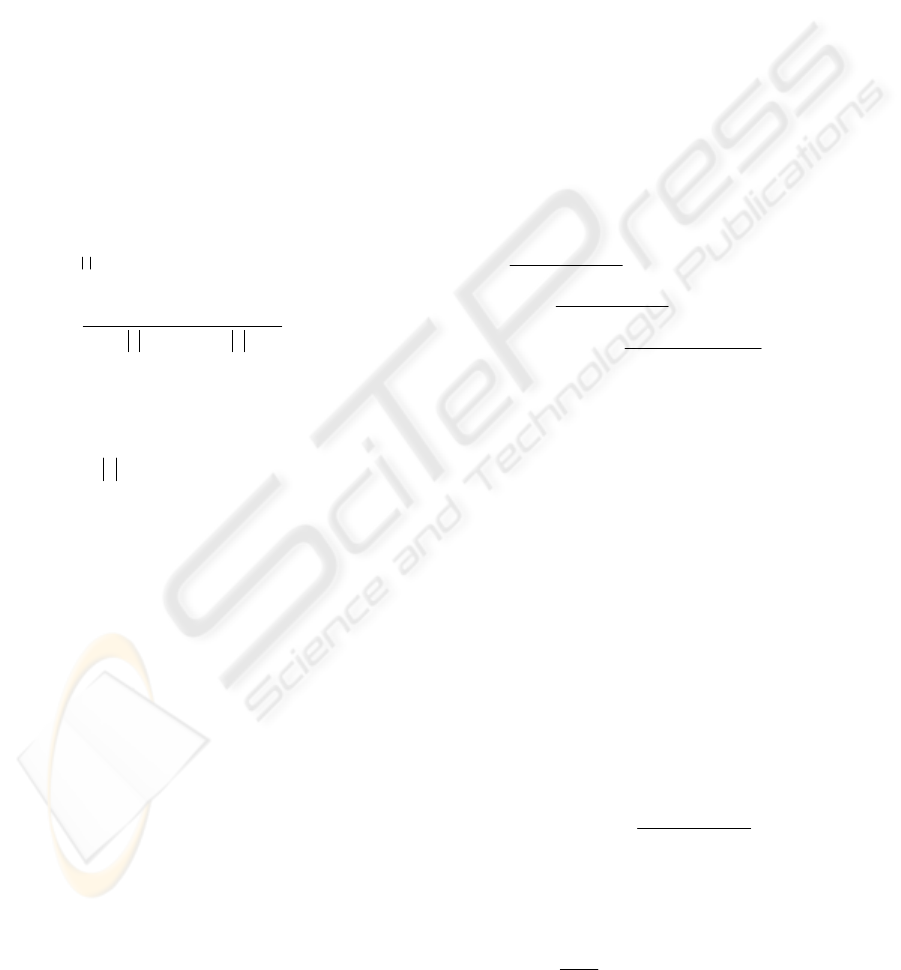
3 MOMENT COMPRESSION
In this section a predefined algorithm that consists of
two complementary paths, involving moment
computation and a compression method, is
presented.
In Fig.1 this algorithm is depicted in a generic
form, in order to maintain a systematic procedure
that performs a feature extraction method, while the
inverse process is also provided.
The concerned algorithm, which is presented in
details in (Papakostas, 2002, 2004), can be
summarized in the following steps:
Direct path
Step 1: The original image is being pre-
processed, (filtering, binarization).
Step 2: Computation of the orthogonal
moments to be compressed, with the
additional ensuring of translation,
scaling invariance, and finally the
computation of the so called “moment
signal”. This 1-D signal consists of the
resulted moments, in the order they
have been produced.
Step 3: Application of the Wavelet transform,
or an alternative one (Fourier), to the
“moment signal”.
Step 4: Compression by thresholding of the
resulted wavelet (Fourier) coefficients.
Original
Image
Image
Pre-Processing
Transformation
Inverse
Transformation
Image
Post-Processing
Computation of
Orthognal
Moments
Image
Reconstruction
Final
Reconstructed
Image
Normalized
Reconstruction
Error
Compression
Figure 1: Generic compression of moment features.
Inverse path
Step 1: Application of the inverse transform,
upon the compressed coefficients, in
order to construct the compressed
“moment signal”.
Step 2: Image reconstruction using the
compressed moments, by applying the
inverse formula of the corresponding
moment family.
Step 3: Image post-processing, including
mapping into the range [0-255],
binarization or histogram equalization.
The direct path of the above algorithm is applied,
in order to generate feature vectors with an as small
as possible dimension, but with an increasing
amount of image information. The resulted feature
vectors are consisted of wavelet coefficients that
describe the compressed moment signal.
The inverse path being used to verify the
effectiveness of the moment based feature vectors,
by means of the normalized reconstruction error.
ON THE RECONSTRUCTION PERFORMANCE OF COMPRESSED ORTHOGONAL MOMENTS
471

In the present paper, the above direct path of the
algorithm is applied to the three sets of orthogonal
moments that have been already presented, and three
feature vectors are obtained. The resulted feature
vectors are compared to each other, by computing
their respective normalized reconstruction errors,
through the inverse path of the algorithm.
4 EXPERIMENTAL STUDY
In this section, the reconstruction performance of the
three moment families, are presented and compared
to each other.
For the present experiments, the wavelet
transform is used to extract the image coefficients,
which will be compressed by soft thresholding
(Donoho, 1995). The binarization procedure is
performed by thresholding using the Otsu method,
while the reconstruction performance is measured by
means of the normalized reconstruction error (Teh,
1988), defined as
() () []
() []
∑∑
∑∑
′
−
=
ij
ij
jif
jifjif
e
2
2
2
,
,,
(19)
where f(i,j) is the intensity function of the
original image and f’(i,j) the intensity function of
the reconstructed one.
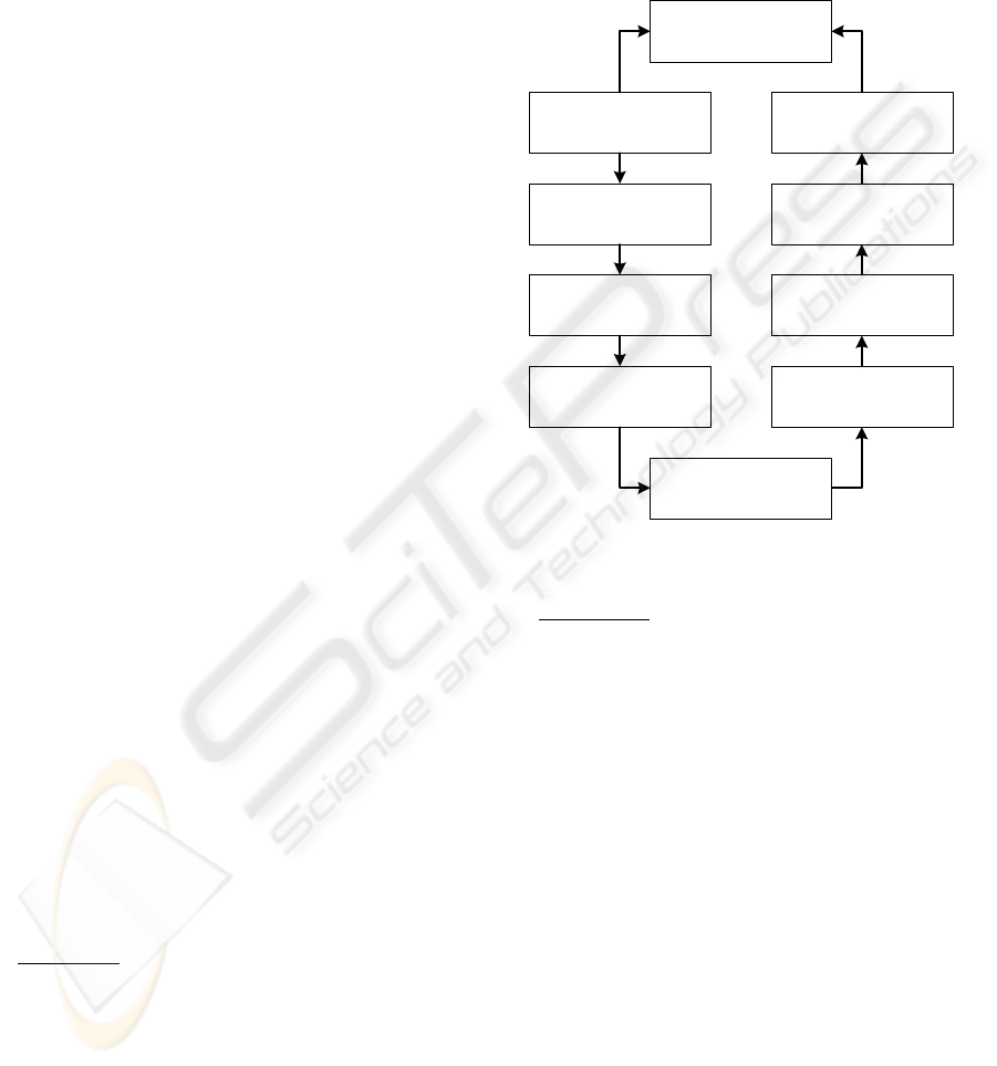
In Figure 2, the mean normalized reconstruction
error for the set of images used in (Papakostas,
2004), for each one of the families of orthogonal
moments, is illustrated.
As can be seen, in the case of Zernike moments
the compression method yields to a set of more
efficient feature vectors, since for the same number
of features the corresponding error is smaller than
that of the uncompressed ones
.
Figure 2: Uncompressed vs Compressed (a) Zernike, (b)
Pseudo-Zernike and (c) Fourier-Mellin moments.
ICINCO 2004 - ROBOTICS AND AUTOMATION
472

(a) (b)
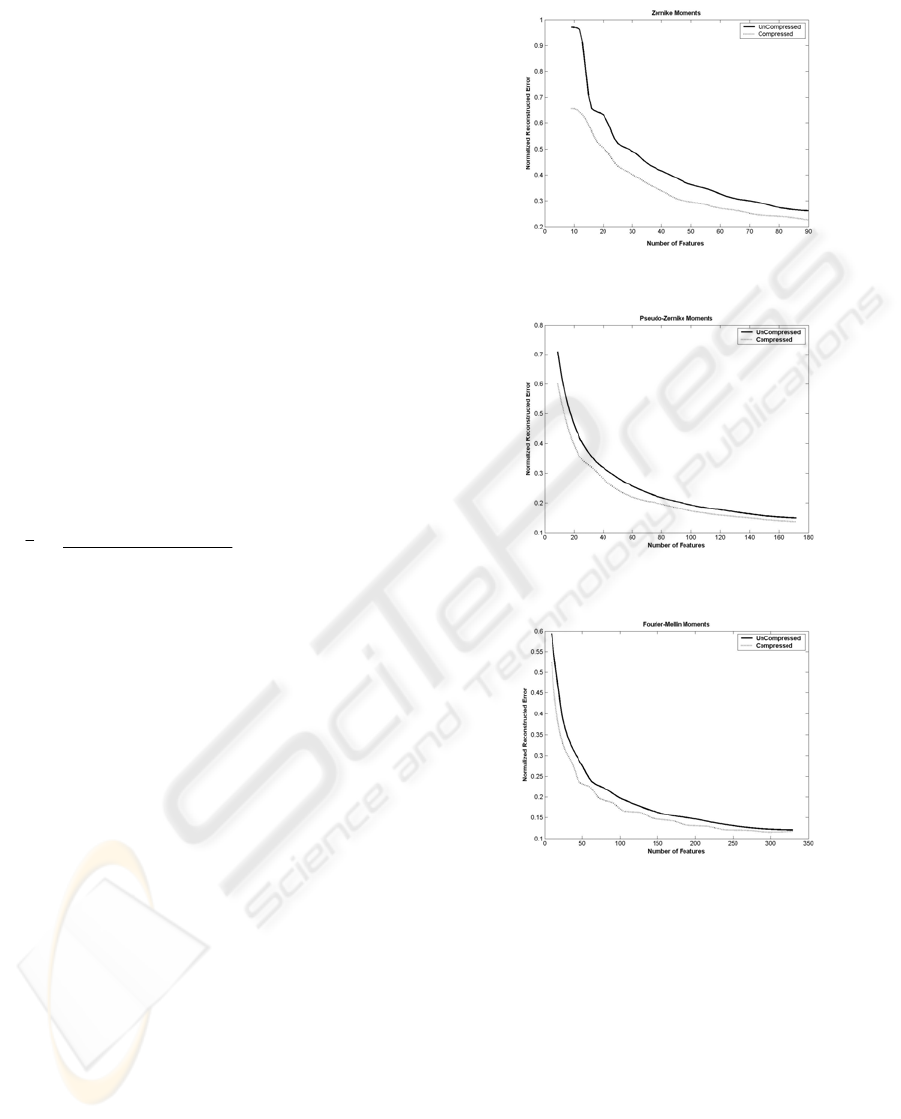
Figure 3: Zernike, Pseudo-Zernike and Fourier-Mellin moments (a) uncompressed, (b) compressed.
In a sense the “moment signals” consisted of the
Zernike moments, have some kind of quantization
error, appeared as noise in the high frequency bands,
and the application of the compression method
operates as denoising. This can be verified by the
fact that Zernike moments are very sensitive to the
presense of noise.
This affect is appeared in a smaller amount in
Pseudo-Zernike and Fourier-Mellin moments, with
the last ones being the most robust noise of all.
Additionaly, Figure 2 points that the proposed
algorithm can be applied successfuly, in all
orthogonal moments keeping the appropriate image
information for the reconstruction of the initial
image with minimum reconstruction error.
Finally, Figure 3 shows that the compression
method improves the reconstruction ability of
Fourier-Mellin moments more than the Pseudo-
Zernike one.
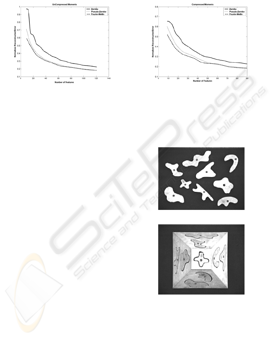
For the above experiments some test objects
(patterns) are initially selected. Figure 4b shows a
wooden pyramidal puzzle, which is used for robot
vision tasks in the Control Systems Lab of DUTH.
The nine parts of the puzzle, placed in arbitrary
positions, are shown in figure 4a. The (256x256)
images of these parts are the nine patterns of our
experiments.
5 CONCLUSIONS
An investigation of the performance of a
compression-based algorithm, to moment signals
derived from three different families of orthogonal
moments, was presented in the previous sections.
The performance was measured, subject to the
reconstruction error that the compressed moments
resulted.
Fourier-Mellin moments seem to improve their
ability in representing an image by a set of
compressed feature moments, better than the other
two families.
(a)
(b)
Figure 4: The nine work pieces that are placed (a) in
arbitrary positions on the table and (b) on a 3-D truncated
pyramid.
The performance of the compressed Pseudo-Zernike
moments remains quite the same to this of the
uncompressed ones, while the application of
compression to the
Zernike moment signal can be
considered as denoising, by removing the high
frequency components.
ON THE RECONSTRUCTION PERFORMANCE OF COMPRESSED ORTHOGONAL MOMENTS
473

REFERENCES
Chong Chee-Way, Mukundan R., Raveendran P., 2001.
“An efficient Algorithm for fast computation of
Pseudo-Zernike Moments”, International conference
on Image and Vision Computing – (IVVCNZ’01), pp.
237-242, New Zealand.
Chong Chee-Way, Raveendran P., Mukundan R., 2003. “
A comparative analysis of algorithms for fast
computation of Zernike moments”, Pattern
Recognition 36, pp. 731-742.
Donoho D.L., 1995. “De-noising by soft-thresholding,”,
IEEE Trans. on Inf. Theory, vol. 41, No. 3, pp. 613–
627.
Hu M.K., 1962. “Visual pattern recognition by moment
invariants”, IRE Trans. Inform. Theory, vol. IT-8, pp.
179-187.
Kan C., Srinath M.D., 2002. “Invariant character
recognition with Zernike and orthogonal Fourier-
Mellin moments”, Pattern Recognition 35, pp. 143-
154.
Khotanzad A. and Hong Y.H., 1990. “Invariant Image
Recognition by Zernike Moments”, IEEE Trans. on.
Pattern Anal. Machine Intell., vol. PAMI-12, No.5.,
pp. 489-497.
Mukundan R., Ramakrishnan K.R., 1995. “Fast
computation of Legendre and Zernike moments”,
Pattern Recognition 28 (9), pp. 1433-1442.
Papakostas G.A., Karras D.A., Mertzios B.G., 2002.
“Image Coding Using a Wavelet Based Zernike
Moments Compression Technique”, 14th International
Conference on Digital Signal Processing (DSP2002),
vol. II, pp. 517-520, 1-3 July 2002, Santorini-Hellas
(Greece).
Papakostas G.A., Karras D.A., Mertzios B.G. and
Boutalis Y.S., 2004. “Pattern Classification by
Wavelet Based Compressed Zernike Moments”,
submitted to EURASIP Journal of Applied Signal
Processing.
Teh C.-H. and Chin R.T., 1988. “On Image Analysis by
the Methods of Moments”, IEEE Trans. on. Pattern
Anal. Machine Intell., vol. PAMI-10, No.4. pp. 496-
513.
ICINCO 2004 - ROBOTICS AND AUTOMATION
474