AUTOMATIC VISION-BASED MONITORING OF THE

SPACECRAFT DOCKING APPROACH WITH THE

INTERNATIONAL SPACE STATION

Andrey A. Boguslavsky, Victor V. Sazonov, Sergey M. Sokolov

Keldysh Institute of Applied Mathematics Russian Academy of Sciences, Miusskaya Sq.4, Moscow, 125047, Russia

Alexandr I. Smirnov, Khamzat S. Saigiraev

S.P. Korolev Rocket & Space corporation “ENERGIA” PLC, 4A Lenin str, Korolev, Moscow area 141070, Russia

Keywords: Real-time vision system, space docking, Vision systems software, algorithms of determining the motion

parameters

Abstract: The software package which allows to automate the visual monitoring of the spacecraft docking approach

with the international space station is being considered. The initial data for this com

plex is the video signal

received from the TV-camera, mounted on the spacecraft board. The offered algorithms of this video signal

processing in real time allow to restore the basic characteristics of the spacecraft motion with respect to the

international space station. The results of the experiments with the described software and real video data

about the docking approach of the spacecraft Progress with the International Space Station are being

presented. The accuracy of the estimation of the motion characteristics and perspectives of the use of the

package are being discussed.

1 INTRODUCTION

One of the most difficult and crucial stages in

managing the flights of space vehicles is the process

of their docking approach. The price of a failure at

performing of this process is extremely high. The

safety of crew, station and space vehicles also in

many respects depends on a success of its

performance.

The radio engineering means of the docking

approach, whi

ch within many years have been used

at docking of the Russian space vehicles, are very

expensive and do not allow to supply docking to not

cooperated station.

As reserve methods of docking approach

m

onitoring the manual methods are applied, for

which in quality viewfinders the optical and

television means are used. For docking approach of

the pilotless cargo transport vehicle Progress to the

orbital station Mir a teleoperation mode of manual

control (TORU) was repeatedly used, at which

realization the crew of the station, having received

the TV image of the station target from a spacecraft,

carried out the manual docking approach.

At the center of the flight management the

cont

rol of objects relative motion parameters (range,

speed, angular deviations) should also be carried

out. The semi-automatic TV methods of the

monitoring which are being used till now, do not

satisfy the modern requirements anymore. Recently

appeared means of both the methods of the visual

data acquisition and processing provide an

opportunity of the successful task decision of a

complete automatic determination and control of

space vehicles relative motion parameters.

The variant of a similar complex (determining

param

eters of the docking approach of the

spacecraft (SC) with the International Space Station

(ISS), on the TV image) is being described below.

The program complex for an automation of the

vi

sual control of the docking process of the SC with

the ISS (further for brevity - complex) is intended to

process in real time on the computers such as IBM

PC the ISS TV-image, transmitted with the camera

onboard SC, with the purpose of the SC and ISS

79

Boguslavsky A., Sazonov V., Sokolov S., Smirnov A. and Saigiraev K. (2004).

AUTOMATIC VISION-BASED MONITORING OF THE SPACECRAFT DOCKING APPROACH WITH THE INTERNATIONAL SPACE STATION.

In Proceedings of the First International Conference on Informatics in Control, Automation and Robotics, pages 79-86

DOI: 10.5220/0001142700790086

Copyright

c

 SciTePress

relative location definition. The TV-signal is

inputted into computer with the help of the

framegrabber. Besides that, the opportunity of the

processing already digitizing of sequences of the avi

format images is stipulated. All complex is realized

in OS Windows 98-XP.

An ultimate goal of the complex development is

a complete automation of the visual monitoring of

SC and ISS docking approach from the moment of

ISS visibility in the TV-camera field of view (about

500 m) and up to the complete SC and ISS docking.

In the basic integrated steps - stages of the

acquisition and processing of the visual data the

complex works similarly to the operator - person.

The complex in addition (in relation to the

person - operator) calculates and displays in the

kind, accepted for the analysis, parameters

describing the docking process.

This research work was partially financed by the

grants of the RFFI ## 02-07-90425, 02-01-00671,

MK-3386.2004.9 and the Russian Science Support

Foundation.

2 MEASURING SUBSYSTEM

The purpose of this software subsystem is the

extraction of the objects of interest from the images

and performance of measurements of the points’

coordinates and sizes of these objects. To achieve

this purpose it is necessary to solve four tasks:

1) Extraction of the region of interest (ROI)

position on the current image.

2) Preprocessing of the visual data inside the

ROI.

3) Extraction (recognition) of the objects of

interest.

4) Performing of the measurements of the sizes

and coordinates of the recognized objects.

All the listed above operations should be

performed in real time. The real time scale is

determined by the television signal frame rate. The

other significant requirement is that in the

considered software complex it is necessary to

perform updating of the spacecraft motion

parameters with a frequency of no less than 1 time

per second.

For reliability growth of the objects of interest

the extraction from the images of the following

features are provided:

1) Automatic adjustments of the brightness and

contrast of the received images for the optimal

objects of interest recognition.

2) Use of the objects of interest features of the

several types. Such features duplication (or even

triplication) raises reliability of the image processing

when not all features are well visible.

3) Self-checking of the image processing results

on a basis of the a priori information about the

observed scenes structure.

The ways of performing the calculation of the

ROI position on the current image are:

1) Calculation of the ROI coordinates (fig. 1) on

the basis of the external information (for example,

with taking into account a scene structure or by the

operator selection).

2) Calculation of the ROI coordinates and sizes

on the basis of the information received from the

previous images processing.

The second (preprocessing) task is solved on the

basis of the histogram analysis. This histogram

describes a brightness distribution inside the ROI.

The brightness histogram should allow the reliable

transition to the binary image. In the considered task

the brightness histogram is approximately bimodal.

The desired histogram shape is provided by the

automatic brightness and contrast control of the

image source device.

(a)

(b)

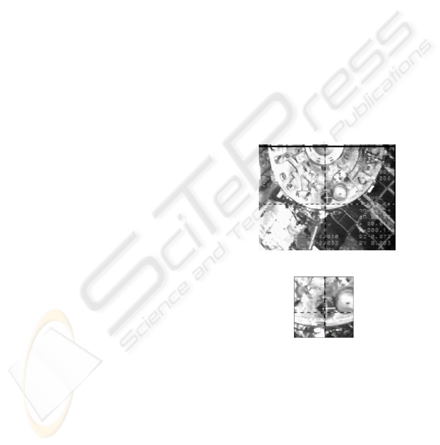
Figure 1: An example of the ROI positioning in the

spacecraft TV-camera field of view. a) Full image of the

field of view; b) The ROI image.

At the third processing stage the extraction of the

objects of interest is performed. These objects are

the station contour, the docking unit disk, the target

cross and the target disk with small labels. The main

features are the station contour, the cross and the

target labels. These features are considered the main

structured elements of the recognized scene and

used for measurement. At features extraction both

edge-based (Canny, 1986; Mikolajczyk et al., 2003)

ICINCO 2004 - ROBOTICS AND AUTOMATION

80

and region-based methods are used (Sonka et al.,

1999).

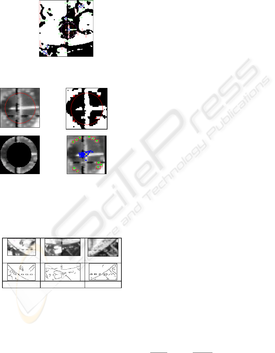
Figure 2: Selection of a cross among all target candidates

on a basis of the a priori information (the sizes of the cross

rods and their relative arrangement).

(a) (b)

(c) (d)

Figure 3: Example of the target labels extraction on the

basis of the target cross coordinates and a priori

knowledge about the labels arrangement. (a) Estimation of

the ROI placement for the labels recognition. (b) Coarse

estimation of the target radius by the diagonal fragments

processing. (c) Ring-shaped ROI with the target labels.

(d) Results of the target labels recognition and the

improved estimation of the target radius.

(a) (b) (c)

Figure 4: Example of the station contour recognition.

(a) The fragment from the left part of the station image.

(b) The fragment from the central part. (c) The fragment

from the right part.

The fourth operation (performing of the

measurement) is very straightforward. But for this

operation it is necessary to recognize the reliable

objects results from the previous processing stages.

3 CALCULATION PART

Preprocessing of a frame (more exactly, a half-

frame) gives the following information:

T

– reference time of a frame (in seconds from a

beginning of video data input);

CC

YX ,

– coordinates of the center of the cross

on the target (real numbers);

1

N

– number of couples of points on the

horizontal crossbar of the cross (integers);

),,2,1(,

1

NiYX

ii

K

=

– coordinates of points

on the top of the horizontal crossbar of the cross

(integers);

),,2,1(,

1

NiYX

ii

K

=

′

– coordinates of points

on the bottom of the horizontal crossbar of the cross

(integers);

2

N

– number of couples of points on the

vertical crossbar of the cross (integers);

),,2,1(,

2

NiVU

ii

K

=

– coordinates of points

on the left side of vertical crossbar of the cross

(integers);

),,2,1(,

2

NiVU

ii

K

=

′

– coordinates of points

on the right side of vertical crossbar of the cross

(integers);

RYX

OO

,,

– coordinates of the center of the

circle on the target and its radius (real numbers);

),,2,1(,,

33

NiBAN

ii

K

=

– number of points

on the circle and their coordinates (integers);

SSS

RYX ,,

– coordinates of the center of the

circle, which is the station outline, and its radius

(real numbers).

Here all coordinates are expressed in pixels.

Some numbers of

can be equal to zero.

For example, the equality

means the

absence of the data

, . Successful

preprocessing a frame always gives the values of

and , but if there is an

opportunity, when appropriate

, those

quantities are determined once again by original

information. Bellow we describe the calculation of

those quantities in the case when

and . If differs

from zero, the data are used in other way (see

bellow).

321

,, NNN

0

1

=N

i

X

i

Y

CC

YX , RYX

OO

,,

0>

k

N

0,0,0

321

>>> NNN 0=

S

R

S

R

Determining the coordinates of the cross center.

We change the data

i

ii

Y

YY

→

′

+

2

,

i

ii

U

UU

→

′

+

2

),2,1( K=i

AUTOMATIC VISION-BASED MONITORING OF THE SPACECRAFT DOCKING APPROACH WITH THE

INTERNATIONAL SPACE STATION

81

and get coordinates of two sequences of points,

which lie in centerlines of horizontal and vertical

crossbars of the cross. Those centerlines have

equations

(horizontal) and

1

cyax =−

2

cayx

=

+

(vertical). Here

, and are coefficients. The

form of the equations takes into account the

orthogonality of these lines. The coefficients are

determined by minimization of the quadratic form

a

1

c

2

c

∑∑

==

+++−−

21

1

2

1

2

1

)()(

N

j

jj

N

i

ii

caVUcYXa

on

, i.e. by solving the linear least squares

problem. The coordinates of the cross center are

21

,, cca

2

21

*

1 a

cac

X

C

+

=

,

2

21

*

1 a

acc

Y

C

+

−

=

.

As a rule,

and do not

exceed 1.5 pixels.

||

*

CC

XX − ||

*

CC

YY −

Determining the radius and the center of the

target circle is realized in two stages. In the first

stage, we obtain preliminary estimations of these

quantities based on elementary geometry. In the

second stage, we solve the least squares problem

minimizing the expression

()()

∑

=

⎥

⎦

⎤

⎢

⎣

⎡

−−+−=Φ

3

1

2

22

2

N

i

OiOi

RYBXA

on

by Gauss-Newton method [1]. Let its

solution be

. As a rule,

||

and

do not exceed 1.5 pixels. Below for

simplicity of notations, we will not use an asterisk in

designations of recomputed parameters.

RYX

OO

,,

***

,, RYX

OO

*

OO

XX −

||

*

OO

YY −

3.1 Basic geometrical ratios

We use the right Cartesian coordinate system

, which is connected with the target. The

point

is the center of the target circle, the axis

is directed perpendicularly to the circle plane

away from station, i.e. is parallel a longitudinal axis

of the Service module, the axis

intersects a

longitudinal axis of the docking device on the

Service Module. Also, we use right Cartesian

coordinate system connected with the TV

camera on the spacecraft. The plane

is an

image plane of the camera, the axis

is a camera

optical axis and directed on movement of the

spacecraft, the axis

intersects an axis of the

docking device of the spacecraft. Let

be the

transition matrix from the system

to the

system

. The transition formulas are

321

yyCy

C

3

Cy

+

2

Cy

321

xxSx

21

xSx

3

Sx

−

2

Sx

3

1,

||||

=ji

ij

a

321

xxSx

321

yyCy

)3,2,1(

3

1

=+=

∑

=

ixady

j

jijii

,

∑

=−= )3,2,1()( jadyx

ijiij

.

Here

are coordinates of the point

in the system

.

321

,, ddd S

321

yyCy

The matrix characterizes ideal docking

)1,1,1(diag||||

−

=

ij

a

. In actual docking the

transition matrix is

1

||||

12

13

23

−−

−

=

ϕϕ

ij

a

where

32

,,

ϕ

are components of the vector of an

infinitesimal rotation of the system

with

respect to its attitude in ideal docking. We suppose

deviations from ideal docking are small.

321

xxSx

If any point has in the system

the

coordinates

, its image has in the image

plane of the camera the coordinates

321

xxSx

),,(

321

xxx

3

1

x

fx

=

ξ

,

3

2

x

fx

=

ξ

.

Here

is focal length of the camera. The

coordinates

f

1

ξ

and

2

ξ

, expressed in pixels, were

meant in the above description of processing a

single video frame. Let coordinates of the same

point in the system

be . Then

321

yyCy

),,(

321

yyy

333323221311

333222111

)()()(

adyadyady

f

iii

i

−+−+−

=

ξ

)2,1(

=

i

The coordinates of the point

C (the center of the

target circle) in the system

are ,

therefore

321

y yCy

)0,0,0(

31221

23321

ddd

fX

O

−+

+−

=

ϕϕ

,

31221

13231

ddd

fY

O

−+

++

−=

ϕϕ

.

In docking

31

|| dd

<

, , so it is

possible to use the simplified expressions

32

|| dd <<

2

3

1

ϕ

f

d

fd

X

O

−−=

,

1

3

2

ϕ

f

d

fd

Y

O

+=

.

ICINCO 2004 - ROBOTICS AND AUTOMATION

82

The center of the cross in the system

has the coordinates

. In this case under the

similar simplification, we have

321

yyCy

),0,0( b

2

3

1

ϕ

f

bd

fd

X

C

−

−=

,

1

3

2

ϕ

f

bd

fd

Y

C

+

−

=

.

So

)

3

(

3

1

bdd

bdf

O

X

C

X

−

−=−

,

)

3

(

3

2

bdd

bdf

O

Y

C

Y

−

=−

.

The radius

r

of the target circle and radius

of its image in the image plane are connected by the

ratio

R

3

d

fr

R =

.

The last three ratios allow to express

, and

through , and . Then it is

possible to find

3

d

1

d

2

d

R

OC

XX −

OC

YY −

1

ϕ

and

2

ϕ

, having solved

concerning these angles the expressions for

or

. As to the angle

OO

YX ,

CC

YX ,

3

ϕ

, the approximate

ratio

a=

3

ϕ

takes place within the framework of

our consideration.

The processing a frame is considered to be

successful, if the quantities

ii

d

ϕ

,

were

estimated. As a result of successful processing a

sequence of frames, it is possible to determine

spacecraft motion with respect to the station. The

successfully processed frames are used only for

motion determination.

)3,2,1( =i

3.2 Algorithm for determination of

the spacecraft motion

The spacecraft motion is determined in real time as a

result of step-by-step processing of a sequence of

TV images of the target. The data are processed by

separate portions. The portions have a fixed volume

or they are formed by the data gathered on time

intervals of fixed length. In the processing of the

second and subsequent portions, the results of

processing of the previous portions are taken into

account.

In each portion is processed in two stages. The

first stage consists in determining the motion of the

spacecraft center of mass; the second stage consists

in determining the spacecraft attitude motion.

Mathematical model of motion is expressed by

formulas

tzzd

211

+

=

,

tzzd

432

+

=

,

tzzd

653

+

=

,

tvv

211

+

=

ϕ

,

tvv

432

+

=

ϕ

,

tvv

653

+

=

ϕ

.

Here

is time counted off the beginning of

processing the frame sequence,

and are

constant coefficients. The ratios written out have the

obvious kinematical sense. We denote the values of

the model coefficients, obtained by processing the

portion of the data with number

n

, by ,

and the functions

,

t

i

z

j

v

)(n

i

z

)(n

j

v

)(td

i

)(t

i

ϕ

, corresponding to

those coefficients, by

, .

)(

tD

n

i

)(

)

t

n(

i

Φ

Determining the motion consists in follows. Let

there be a sequence of successfully processed

frames, which correspond to the instants

...

321

<

ttt

. The frame with number

corresponds to the instant

. Values of the

quantities

, , , , , , which were

found by processing this frame, are

, , etc.

These values with indexes

form the

first data portion, the value with indexes

k

t

C

X

C

Y a

O

X

O

Y R

)(k

C

X

)(k

C

Y

1

,,2,1 Kk K=

211

,,2,1 KKKk K

+

=

– the second one, with

indexes

nnn

KKKk ,,2,1

11

K+

+

=

−−

– the -th

portion.

n

The first data portion is processed by a usual

method of the least squares. The first stage consists

in minimization of the functional

∑

=

=Ψ

1

)(

K

k

Az ,

+

⎥

⎦

⎤

⎢

⎣

⎡

−

+−=

2

)(

3

)(

3

)(

1

)()(

1

][ bdd

bdf

XXwA

kk

k

O

k

C

k

+

⎥

⎦

⎤

⎢

⎣

⎡

−

−−

2

)(

3

)(

3

)(

2

)()(

2

][ bdd

bdf

YYw

kk

k

O

k

C

2

)(

3

)(

3

⎥

⎦

⎤

⎢

⎣

⎡

−

k

d

fr

Rw

.

Here

, is a vector

of the coefficients, which specify the functions

, , is positive numbers (weights). The

minimization is carried out by Gauss -Newton

method [1]. The estimation

)(

ki

k

i

tdd =

T

zzzz ),,,(

621

K=

)(td

i i

w

)1(

z

of

z

and the

covariance matrix

of this estimation are defined

by the formulas

1

P

[

]

)(minarg,,,

1

)1(

6

)1(

2

)1(

1

)1(

zzzzz

T

Ψ== K

,

AUTOMATIC VISION-BASED MONITORING OF THE SPACECRAFT DOCKING APPROACH WITH THE

INTERNATIONAL SPACE STATION

83

1

2

1

−

= BP

σ

,

[

]

63

1

)1(

1

2

−

Ψ

=

K

z

σ

.

Here

is the matrix of the system of the normal

equations arising at minimization of

. The matrix

is calculated at the point

1

B

1

Ψ

)1(

z

.

At the second stage, the quantities

⎥

⎦

⎤

⎢

⎣

⎡

−=

)(

1

)1(

3

)1(

2

)()(

1

k

O

k

tD

tfD

Y

f

α

,

⎥

⎦

⎤

⎢

⎣

⎡

+−=

)(

1

)1(

3

)1(

1

)()(

2

k

O

k

tD

tfD

X

f

α

are calculated and three similar linear regression

problems

k

tvv

21

)(

1

+≈

α

, ,

k

tvv

43

)(

2

+≈

α

k

tvva

65

)(

+≈

),,2,1(

1

Kk K=

are solved using the standard least squares method

[2]. We content ourselves with description of

estimating the couple of parameters . We

unite them in the vector

. The

estimations

and provide the minimum to

the quadratic form

21

, vv

T

vvv ),(

21

=

)1(

1

v

)1(

2

v

[]

2

1

21

)(

1

)(

∑

=

−−=

K

k

tvvvF

α

.

Let

be the matrix of this form. Then the

covariance matrix of the vector

is

.

1

Q

T

vvv ],[

)1(

2

)1(

1

)1(

=

)2/(][

1

)1(

1

−

KvFQ

The second data portion is carried out as follows.

At the first stage, the functional

[][]

∑

+=

+−−=Ψ

2

1

)1(

2

)1(

2

)(

K

Kk

k

T

AzzCzzz

is minimized. Here

12

qBC

=

, is a parameter,

. The estimation of

q

10 ≤≤ q

z

and its covariance

matrix have the form

)(minarg

2

)2(

zz Ψ=

, ,

1

2

−

= BP

σ

[]

6)(3

12

)2(

2

−−

Ψ

=

KK

z

σ

,

where

is the matrix of the system of the normal

equations, which arise at minimization of

2

B

2

Ψ

,

calculated at the point

)2(

z

.

At the second stage, the quantities

and

(see above) are calculated and the estimation

of the coefficients

are found. The estimation

provides the minimum to the quadratic form

)(

1

k

α

)(

2

k

α

)2(

j

v

)2(

v

[

][ ]

+−−

′

=

)1(

1

)1(

2

)( vvQvvqvF

T

[]

2

1

21

)(

1

2

1

∑

+=

−−

K

Kk

k

tvv

α

.

Here

q

′

is a parameter, . Let be the

matrix of this form. The covariance matrix of the

estimation

is .

10 ≤

′

≤ q

2

Q

)2(

v

)2/(][

12

)2(

2

1

2

−−

−

KKvFQ

The third and subsequent data portions are

processed analogously to the second one. The

formulas for processing the portion with number

are obtained from the formulas for processing the

second portion by replacement of the indexes

expressed the portion number:

, .

n

11 −→ n n→2

The described algorithm is rather similar to

nonlinear Kalman filter. The matrix

in Kalman

filter (compare the above

) is defined by the

formula

. Here is the

covariance matrix of the term in the difference

n

C

2

C

1

)(

−

+=

nnn

GPC

n

G

)1()( −

−

nn

z

, which is caused by errors in the

mathematical model at transition from the time

interval

12

1

−−

≤

+

nn

KK

ttt

to the interval

nn

KK

ttt

≤

+

−

1

. Our choice of and

n

C )(z

n

Ψ

means that the covariance matrix of errors in

OC

XX

−

,

OC

YY

−

and is equal to

.

R

),,(diag

1

3

1

2

1

−−−

www

It is easy to see that

, i.e. the matrix

1−

<

nn

BC

nn

CB

−

−1

is positive definite. The introduction of

the matrix

provides diminution of influence of

the estimation

n

G

)1( −n

z

on the estimation

)(n

z

.

Unfortunately, the matrix

is unknown. In such

situation, it is natural to take

. One has

n

G

1−

=

nn

qBC

1−

<

nn

BC

if

1

<

q

. The described choice of

means, that procession of the

n

-th data portion

takes into account the data of the previous portions.

The data of the

-th portion are taken in processing

with the weight 1, the

n

C

n

)1(

−

n

-th portion is attributed

the weight

, the

q )2(

−

n

-th portion has the weight

, etc.

2

q

The results of processing the

-th data portion

are represented by numbers

,

n

)(

n

K

n

i

tD

)(

n

K

n

i

tΦ

),2,1;3,2,1( K

=

ni

. We calculate also the

quantities

ICINCO 2004 - ROBOTICS AND AUTOMATION

84

2

3

2

1

ddd ++=

ρ

,

d

t

d

u

ρ

=

,

2

3

2

1

2

arctan

dd

d

+

=

α

,

3

1

arctan

d

=

β

.

The angle

α

is called a passive pitch angle, the

angle

β

is a passive yaw angle. If docking is close

to ideal (considered case), then

31

|| dd

<

,

and

32

|| dd <<

3

2

d

=

α

,

3

1

d

=

β

.

The angle

1

ϕ

is called an active pitch angle,

2

ϕ

is an active yaw angle,

3

ϕ

is an active roll angle.

We remind these angles have small absolute values.

Characteristics of accuracy of the motion

parameter estimations are calculated within the

framework of the least squares method. For

example, we defined above the covariance matrix

of the estimation

n

P

)(n

z

. In terms of this matrix

the covariance matrix

of the vector

)(tC

w

=

)(tw

is

calculated by formulas

(

12

665443221

,,,,,, Rvtvvztzzztzz

T

∈+++ K

)

T

nw

z

w

P

z

w

C

⎟

⎠

⎞

⎜

⎝

⎛

∂

=

U)U,(U,diag=

∂

z

w

,

00

1 t

U =

.

These formulas concern to the motion which was

found by processing the -th of a portion of the

data.

n

Knowing

, it is possible to calculate the

standard deviations

)(tC

w

)(t

ρ

σ

,

)(t

u

σ

,

)(t

α

σ

and

)(t

β

σ

of the quantities

)(t

ρ

, ,

)(tu )(t

α

and

)(t

β

.

The standard deviation

)(t

ρ

σ

has the form

T

w

C

w

⎟

⎠

⎞

⎜

⎝

⎛

∂

=

ρρ

σ

ρ

,

T

d

dd

w

⎟

⎠

⎞

⎜

⎝

⎛

=

∂

ρρρ

ρ

3

21

,0,,0,

.

The similar formulas define the others standard

deviations. The values of

ρ

,

ρ

σ

, ,

u

σ

, etc.,

referring to the last instant of the processed data

portion, are written on the computer display.

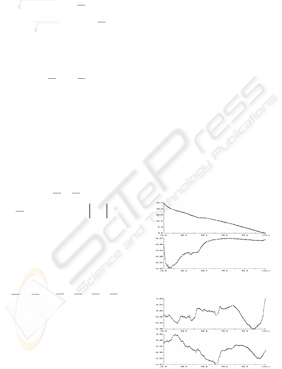
4 EXAMPLES

Fig. 5, 6 give examples of the operation of the

described algorithm estimating the spacecraft

motion. Fig. 5 contains the plots of the functions

)(t

ρ

, ,

)(tu )(t

α

and

)(t

β

and

)(t

i

ϕ

,

fig. 6 presents the plots of the standard deviations

)3,2,1( =i

)(t

ρ

σ

,

)(t

u

σ

,

)(t

α

σ

,

)(t

β

σ

. The values of all

these functions were calculated at the last instants of

processed data portions. These values were shown

by marks. Each portion contained 10 instants with

measurements:

10

1

=

−

−nn

KK

. For clearness, the

markers were connected by segments of straight

lines, therefore presented plots are broken lines.

Only the vertexes of these broken lines are

significant. Their links are only interpolation, which

is used for visualization and not always exact. As it

is shown in fig. 6, the spacecraft motion on the final

stage of docking was defined rather accurately.

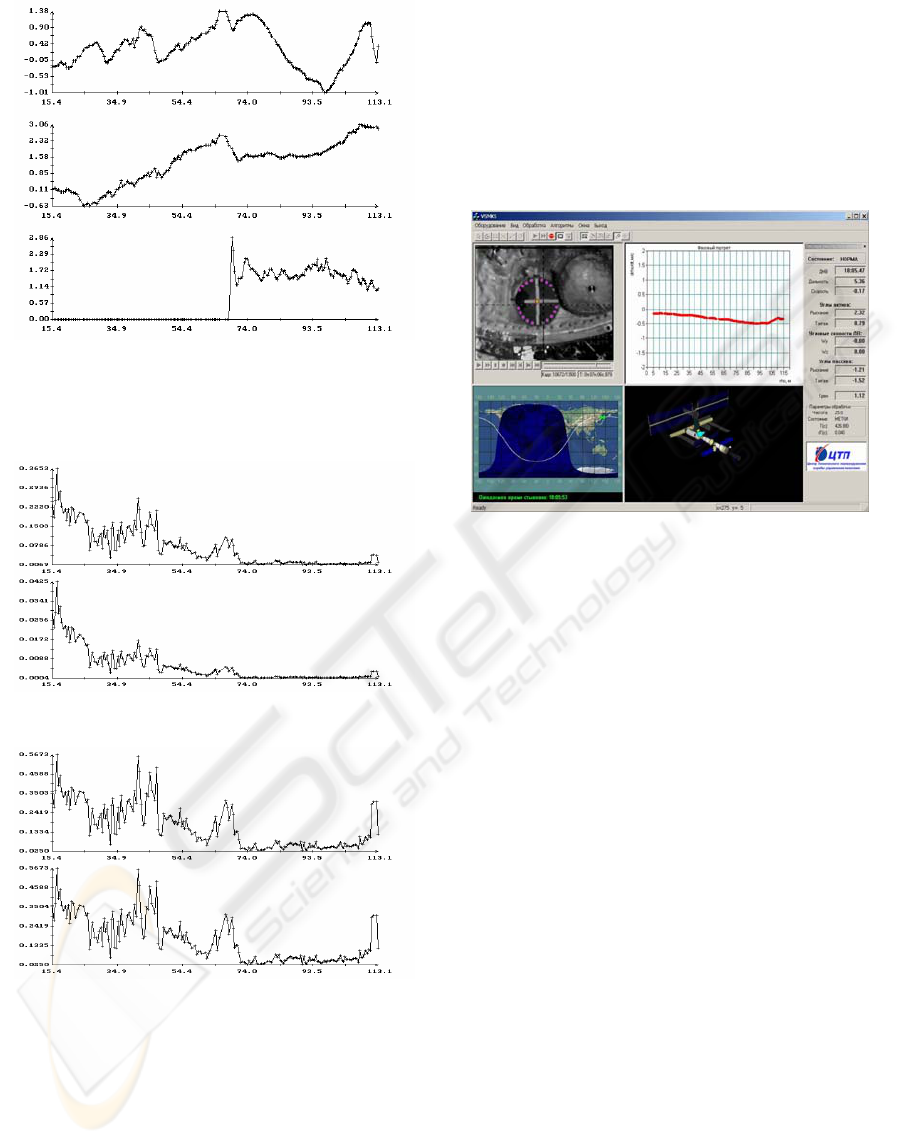
Figure 7 shows an examples of the basic screen

of the main program of a complex.

5 CONCLUSION

The described software package is used now as a

means allowing the ground operators to receive the

information on the motion parameters of the

spacecraft docking to ISS in real time.

ρ

(m), (m/s)

u

t (s)

β

α

,

(deg.)

t (s)

321

,,

ϕ

(deg.)

AUTOMATIC VISION-BASED MONITORING OF THE SPACECRAFT DOCKING APPROACH WITH THE

INTERNATIONAL SPACE STATION

85

t (s)

Figure 5: Results of determination of the spacecraft

motion in docking approach.

ρ

σ

(m),

u

σ

(m/s)

t (s)

βα

σ

,

(deg.)

t (s)

Figure 6. Accuracy estimations for the motion presented

on Fig. 5.

The most essential part of this information is

transferred to the Earth (and was always transferred)

on the telemetering channel. It is also displayed on

the monitor. However this so-called regular

information concerns the current moment and

without an additional processing can’t give a

complete picture of the process. Such an additional

processing is much more complicated from the

organizational point of view and more expensive

than processing the video image. It is necessary to

note, that the estimation of kinematical parameters

of the moving objects on the video signal, becomes

now the most accessible and universal instrument of

solving such kind of problems in situations, when

the price of a failure is rather insignificant.

Figure 7: An example of the monitoring system main

window. The distance is 5.3 meters. The main window is

divided onto four parts. In the top left part the TV-camera

field of view is displayed. In the bottom left part the

ballistic trajectory of ISS and the day and night areas are

shown. In the top right part the phase chart is displayed. In

the bottom right part the 3D model of the ISS and

spacecraft are rendered. In the grey panel (near the right

edge of the main window) the current system parameters

are displayed (the spacecraft speed, distance, orientation

etc.).

REFERENCES

Mikolajczyk, K., Zisserman, A., Schmid, C., 2003. Shape

recognition with edge-based features. In Proc. of the

14th British Machine Vision Conference

(BMVC’2003), BMVA Press, 2003.

Sonka, M., Hlavac, V., Boyle, R. 1999. Image Processing,

Analysis and Machine Vision. MA: PWS-Kent, 1999.

Canny, J. 1986. A computational approach to edge

detection. In IEEE Trans. Pattern Anal. and Machine

Intelligence, 8(6): pp. 679-698.

Yonathan Bard. Nonlinear parameter estimation.

Academic Press. New York - San Francisco - London,

1974.

G.A.F. Seber. Linear regression analysis. John Wiley and

sons, New York - London - Sydney - Toronto, 1977.

ICINCO 2004 - ROBOTICS AND AUTOMATION

86