DYNAMIC ROUTING AND QUEUE MANAGEMENT

VIA BUNDLE SUBGRADIENT METHODS

Almir Mutapcic, Majid Emami and Keyvan Mohajer

Information Systems Laboratory

Stanford University, Stanford, CA 94305

Keywords:

Dynamic network routing, queue management, dual methods, bundle subgradient methods.

Abstract:

In this paper we propose a purely distributed dynamic network routing algorithm that simultaneously regulates

queue sizes across the network. The algorithm is distributed since each node decides on its outgoing link

ﬂows based only on its own and its immediate neighbors’ information. Therefore, this routing method will

be adaptive and robust to changes in the network topology, such as the node or link failures. This algorithm

is based on the idea of bundle subgradient methods, which accelerate convergence when applied to regular

non-differentiable optimization problems. In the optimal network ﬂow framework, we show that queues can

be treated as subgradient accumulations and thus bundle subgradient methods also drive average queue sizes

to zero. We prove the convergence of our proposed algorithm and we state stability conditions for constant

step size update rules. The algorithm is implemented using Matlab and its performance is analyzed on a test

network with varying data trafﬁc patterns.

1 INTRODUCTION

This paper investigates joint dynamic routing and

queue management in data networks. In networking

literature, queue management is often referred to as

congestion control, since congestion in networks oc-

curs when current link capacities cannot satisfy the

user’s needs, and we have to delay the user’s data

packets by storing them in queues. Network perfor-

mance and its Quality of Service (QoS) are measured

by metrics such as routing delay, maximum link uti-

lization, convergence time after failures, etc.

Many current routing algorithms used in practice

are based on heuristics and are not optimal in any

sense. They are often static (ﬁxed-time) algorithms;

they make ﬂow decisions ahead of time and ﬁx all

routing tables for future network use. For example,

most of routing protocols use hop-counts or some ar-

tiﬁcial weights assigned to the links in order to derive

routing tables for a given network.

We will investigate new routing strategies that are

dynamic in time, and that simultaneously optimize

queue lengths in the network. Dynamic routing algo-

rithms continuously change packet routes as the net-

work topology and users’ demands change; for a dy-

namic routing algorithm example see (Segall, 1977).

Routing methods can also be classiﬁed based on the

type of network coordination. We can have central-

ized, synchronously distributed, and asynchronously

distributed algorithms. We are interested in dis-

tributed algorithms since they do not require any cen-

tralized coordinator with a global network knowl-

edge, and they are more robust to adversarial changes

in network topology.

2 OPTIMAL ROUTING AND

QUEUE MANAGEMENT

2.1 Optimal routing

One way to improve routing through network is by us-

ing multiple paths between any pair of source and des-

tination nodes in the network. Current routing meth-

ods like the routing mechanism in the OSPF protocol

utilize this idea in a limited sense, i.e., the data pay-

load is divided among the shortest paths (if more than

one) toward the given destination. This is still not an

optimal solution; however, it is better than using a sin-

gle routing path.

Mutapcic A., Emami M. and Mohajer K. (2004).

DYNAMIC ROUTING AND QUEUE MANAGEMENT VIA BUNDLE SUBGRADIENT METHODS.

In Proceedings of the First International Conference on Informatics in Control, Automation and Robotics, pages 12-19

DOI: 10.5220/0001144800120019

 SciTePress

2.2 Queue management

The main goal of a queue management algorithm is

to maximize throughput and minimize queue delays

in a network. In this case it is highly desirable to have

a distributed queue management algorithm since it is

impossible to coordinate all source nodes in a large

network.

Our routing strategy will optimize average queue

sizes, and therefore implement a dynamic routing

strategy with active queue management.

2.3 Problem formulation

General joint dynamic routing and queue manage-

ment problems can be formulated as a convex opti-

mization problem constrained by a linear dynamical

system and feasibility constraints. This problem is an

instance of the optimal control problem, where our

objective (performance) function can be any convex

function. Using a discrete time queuing model, and

a single user trafﬁc on a connected directed network

with n nodes and p links, we obtain the following

problem

minimize

t=t

j=1

(t))

i=1

(t)) − U (s(t)) ]

subject to q(t + 1) = q(t) + s(t) − Ax(t),

−c ¹ x(t) ¹ c,

0 ¹ q(t) ¹ Q

max

min

¹ s(t) ¹ S

max

Problem variables are: trafﬁc ﬂows x(t) ∈ R

which can have negative components since we allow

reverse ﬂow on the network links (i.e., the links are

bi-directional); queue lengths q(t) ∈ R

represent

amount of packets waiting to be processed at each

node’s queue; source rates s(t) ∈ R

is a vector of

incoming and removed network trafﬁc at each node,

such that

i=1

(t) = 0. The ﬂows are restricted

by the given link capacities c

> 0, the queues size

limit is Q

max

, and the source-sink rates can be varied

between S

min

and S

max

. The matrix A ∈ R

n×p

is the

node incidence matrix for the given directed graph.

The function φ

: R → R is the ﬂow cost function

for link j, ψ

: R → R is the queue size penalty

function for node i, and U : R

→ R is the utility

measure function for a given source-sink rate vector

Typically encountered ﬂow cost functions are

(t)) =

(t)|

− |x

(t)|

, (1)

φ(x(t)) = max

(t)|

where the domain of φ is dom φ

= (−c

, c

The ﬁrst function gives the expected waiting time in

M/M/1 queue, while the second function gives the

maximum link utilization, see (Bertsekas and Gal-

lager, 1991).

Typical queue penalty functions ψ

are linear or

quadratic functions, where later one heavily penalizes

buildup of very large queues.

Utility functions U represent the user utility for dif-

ferent source-sink ﬂows. They show willingness of

the user to pay for an additional amount of network

bandwidth.

An equivalent (relaxed) formulation of the general

problem will be considered in this paper. We will

assume that each customer (node) has an exact net-

work rate agreement, and therefore we can remove

utilization functions from our objective and eliminate

source rate constraints. We will choose the ﬂow cost

functions φ

such that they act as barrier functions for

(t) feasibility. For example, the ﬂow cost functions

from equation (1) can be deﬁned to be ﬁnite inside of

their domain (−c, c) and inﬁnite outside. Therefore,

if we start in the feasible ﬂow region, we will always

stay feasible, and the link capacity constraints will

be automatically enforced. Final relaxation is that

we will not limit queue sizes, since we want to ob-

serve queues behavior especially when they become

unbounded. In practical systems, queues will be ﬁ-

nite and they will start dropping packets when they

become over-saturated. Therefore, our ﬁnal problem

formulation is

minimize

t=t

j=1

(t))

i=1

(t)) ]

subject to q(t + 1) = q(t) + s(t) − Ax(t),

q(t) º 0.

(2)

Since we will only consider convex ﬂow cost and

queue size penalty functions, this is a convex

optimization problem; convex optimization topics

are beautifully treated in (Boyd and Vandenberghe,

2003). Since we have a convex optimization prob-

lem, there exists a global optimal solution which we

will seek to ﬁnd using a dynamical and distributed al-

gorithm.

3 DUAL METHODS

In order to gain some insight into problem (2) in dy-

namical settings, we will ﬁrst investigate its solution

in a static case. We formulate the static-time optimal

network ﬂow problem by setting all queues to zero

for all the time (basically removing queues from the

system) and thus only enforcing the ﬂow conservation

DYNAMIC ROUTING AND QUEUE MANAGEMENT VIA BUNDLE SUBGRADIENT METHODS

constraint in the network.

minimize

j=1

)

subject to Ax = s.

The Lagrangian for this problem is

L(x, ν) =

j=1

) + ν

(s − Ax)

j=1

(φ

) − ∆ν

) + ν

where we interpret the Lagrangian dual variable ν

a potential at node i, and ∆ν

denotes potential differ-

ence across link j. For more details about the optimal

network ﬂow problem, and the following material on

dual decomposition and subgradient methods please

refer to the manuscript (Boyd et al., 2003).

3.1 Dual network ﬂow problem

The dual function is deﬁned as the inﬁmum of La-

grangian over the primal problem variables, and we

have

d(ν) = inf

L(x, ν)

j=1

inf

(φ

) − ∆ν

) + ν

= −

j=1

∗

(∆ν

) + ν

where φ

∗

is the conjugate function of φ

We express the dual network ﬂow problem as

maximize d(ν) = −

j=1

∗

(∆ν

) + ν

which is an unconstrained maximization of a concave

function and we can use appropriate optimization al-

gorithms to obtain an optimal dual solution ν

3.2 Subgradient methods

Since the dual function is a concave, but possibly non-

differentiable function, we will use a subgradient-

based method for its optimization. We will ﬁrst derive

an expression for the subgradients of a negative dual

function.

Consider a dual function for the primal prob-

lem min

(x) subject to the equality constraints

(x) = 0, where i = 1, . . . , n. We will assume f

strictly convex, and denote,

∗

(ν) = argmin

(z) + ν

(z) + · · · + ν

(z))

so the dual function is

d(ν) = f

∗

(ν))+ν

∗

(ν))+· · ·+ν

∗

(ν)).

Then, a subgradient of the negative dual function −d

at ν is given by g

= −f

∗

(ν)). The dual optimiza-

tion method will consist of maximizing the dual func-

tion by stepping in the direction of the subgradient g.

Thus, we obtain the subgradient method optimization

rules for the dual problem:

(k)

= x

∗

(ν

(k)

), ν

(k+1)

= ν

(k)

+ α

(k)

In the case of optimal network ﬂow problem (which

only has equality constraints Ax = s), subgradient at

ν is

g = Ax

∗

(∆ν) − s.

The ith component of subgradient is g

∗

(∆ν) − s

, which is the excess ﬂow at node i,

but also the amount of data that q

would accumulate

after that iteration if we did not remove the queues.

Finally, the original optimal network ﬂow problem

can be solved by applying the subgradient method op-

timization to its dual problem, and then recovering the

primal solutions after the algorithm converges. The

algorithm’s main steps are outlined below:

:= x

∗

(∆ν

)

:= a

x − s

:= ν

− αg

where x

∗

(∆ν

) = argmin

(φ

) − ∆ν

The method proceeds as follows. Given the current

value of node potentials, the ﬂow for each link is lo-

cally calculated. We then compute the ﬂow surplus at

each node. Again, this is local; to ﬁnd the ﬂow sur-

plus at node i, we only need to know the ﬂows on the

links that enter or leave node i. Finally, we update the

potentials based on the current ﬂow surpluses. The

update is very simple: we increase the potential at a

node with a positive ﬂow surplus, which will result in

reduced ﬂow into the node. Provided the step length α

can be computed locally, the algorithm is distributed;

the links and nodes only need information relating to

their adjacent ﬂows and potentials. There is no need

to know the global topology of the network, or any

other nonlocal information, such as what the ﬂow cost

functions are. Since we use the simplest subgradient

update method with constant step sizes α, this algo-

rithm is completely distributed.

Also since we use constant step sizes, this algo-

rithm (if stable) converges to the optimal solution (or

precisely, it converges to the ball of some arbitrary

radius R related to step size α and centered at the op-

timal solution). For more details about this algorithm

and its performance, please see (Boyd et al., 2003).

3.3 Optimal network ﬂow in

dynamic setting

We can apply the optimal network ﬂow algorithm de-

rived in the previous subsection to the problems in a

ICINCO 2004 - INTELLIGENT CONTROL SYSTEMS AND OPTIMIZATION

dynamic setting. Note that now each iteration step k

is the actual time t. The subgradient method ﬁnds the

optimal solution for network ﬂows that satisﬁes the

ﬂow conservation constraint; however, queues accu-

mulate the excess ﬂow data and are not drained after

this initial build-up of data. This scenario is presented

in ﬁgures 1 and 2.

0 50 100 150

−0.3

−0.2

−0.1

0.1

0.2

0.3

0.4

0.5

0.6

Figure 1: Flows x

(t) vs time t with α = 2.5.

0 50 100 150

Figure 2: Queue sizes q

(t) vs time t with α = 2.5.

We see that link ﬂows x

converge to their opti-

mal values (ﬁgure 1), while the queues accumulate

the excess ﬂow until the ﬂow conservation equality is

satisﬁed (ﬁgure 2).

4 BUNDLE SUBGRADIENT

METHOD AND ALGORITHM

We consider a simple modiﬁcation for the static-time

dual subgradient method algorithm derived in the pre-

vious section. In order to discharge the queues we

will linearly add queue lengths q

(t) to the potential

updates ν

(t) in the algorithm. Therefore, our new

potential update step is:

(t + 1) = ν

(t) − α

(t)

(t) + β

(t)

(t).

This modiﬁcation can be interpreted as follows; we

adjust the potential at each node proportional to its

queue size in order to increase the ﬂow out of that

node, while we still step in the direction of nega-

tive dual subgradient, which will reduce the excess

ﬂow (future queue accumulation) for that node. If

the queue size is very large, then we greatly inﬂuence

the link ﬂow out of that node (its queue discharge),

whereas if the queue size is small the link ﬂow will be

mainly determined by balancing of excess ﬂow equa-

tions. This rule should simultaneously decrease the

excess ﬂow and queue lengths, as experimentally ver-

iﬁed in section 6. Also note that our modiﬁcation has

preserved the distributed nature of the algorithm; we

only require local queue information for each node.

The modiﬁed algorithm was applied to the static

case simulation, and the results shown in ﬁgures 3

and 4 verify that queues are discharged after the initial

build-up.

We have obtained an efﬁcient queue regulation us-

ing this new algorithm, and next we will analyze its

theoretical performance.

4.1 Queues are subgradients

As we have already mentioned, queues are accumula-

tions of previous excess ﬂows, which are subgradients

at the previous time points (iterations).

q(t + 1) − q(t) = Ax

∗

(∆ν(t)) − s(t) = g(t).

Assuming zero initial conditions at the start of the

network operation, then at time t = 0, 1, . . . , N , we

have

q(1) = g(0) = Ax

∗

(∆ν(0)) − s(0),

q(2) = g(0) + Ax

∗

(∆ν(1)) − s(1),

q(N + 1) =

N−1

t=0

g(t) + Ax

∗

(∆ν(N )) − s(N).

The original subgradient method iteration for dual

network ﬂow problem is

(k+1)

= ν

(k)

− α

(k)

where ν

(k)

is the voltage at kth iteration, g

(k)

is any

subgradient of −d at ν

(k)

, and α

> 0 is the kth step

size.

At each iteration, the subgradient method uses only

the current subgradient g (the current excess ﬂow or

queue increment at time k).

DYNAMIC ROUTING AND QUEUE MANAGEMENT VIA BUNDLE SUBGRADIENT METHODS

0 50 100 150

−0.4

−0.2

0.2

0.4

0.6

0.8

Figure 3: Flows x

(t) vs t with α = 2.5 and β = 0.2.

0 50 100 150

0.5

1.5

2.5

3.5

Figure 4: Queues q

(t) vs t with α = 2.5 and β = 0.2.

4.2 Subgradient bundle method

We will deﬁne the subgradient bundle method itera-

tion as

(k+1)

= ν

(k)

− α

(k)

where

(k)

k = 0,

(k)

+ β

(k−1)

k > 1.

Here, ν

(k)

is the voltage at kth iteration, g

(k)

is any

subgradient of −d at ν

(k)

, and w

(k)

is the subgradient

bundle (or memory) of −d at kth step. Now we have

two step size constants, α

> 0 is the kth step size

for excess ﬂow update, and β

> 0 is the kth step

size for subgradient bundle. This new algorithm is a

variant of the subgradient bundle method, originally

developed independently by Lamarechal and Wolfe,

see (Lamarechal and Wolfe, 1975).

Switching from iterations k to the actual time t, we

have

w(t) = g(t) + β

(t)

w(t − 1)

= g(t) + β

(t)

˜q(t)

= ˜q(t + 1)

where ˜q(t) = cq(t), c ∈ R

, only if β

(t)

is a constant

step size. If we ﬁx β = 1 for all t, then w(t) is pre-

cisely q(t +1), the queue size at the end of the current

time slot.

Thus, if we take the queue penalty functions to be

linear, ψ(q(t)) = q(t), we are simultaneously solv-

ing the optimal ﬂow problem and minimizing queue

lengths. We can claim that we are searching for the

optimal point of our problem, where the subgradient

is equal to zero, and therefore the queue sizes will be

driven to zero.

5 CONVERGENCE PROOF

In this section, we derive the convergence results for

the bundle subgradient method applied to the optimal

network ﬂow problem.

Let ν

be an optimal dual solution. Deﬁne conver-

gence ranges for step sizes α

and β

0 < α

≤

d(ν

) − d(ν

)

(k)

and

(

−γ

(k)

)

(k−1)

if (g

(k)

)

(k−1)

< 0,

0 otherwise,

where γ ∈ [0, 2].

Using induction we will prove that for step sizes α

and β

satisfying the above convergence conditions,

we have

kν

− ν

(k+1)

k < kν

− ν

(k)

k (3)

and furthermore,

(ν

− ν

(k)

)

(k)

≥

(ν

− ν

(k)

)

(k)

, (4)

so the angle between w

(k)

and ν

− ν

(k)

is no larger

than the angle between g

(k)

and ν

− ν

(k)

Proof: Let d

= d(ν

) be the optimal value of the

dual function. By induction we will ﬁrst show that

(ν

− ν

(k)

)

(k)

≥ (ν

− ν

(k)

)

(k)

, (5)

for all k. We have w

(0)

= g

(0)

, thus it holds for k = 0.

Assuming it holds for k, we will prove it for k + 1.

Since w

(k)

= g

(k)

+ β

(k−1)

, we have

(ν

− ν

(k+1)

)

(k+1)

= (ν

− ν

(k+1)

)

(k+1)

(ν

− ν

(k+1)

)

(k)

ICINCO 2004 - INTELLIGENT CONTROL SYSTEMS AND OPTIMIZATION

and using concavity of the dual function d and step

size convergence conditions, we obtain,

(ν

− ν

(k+1)

)

(k+1)

≥ (ν

− ν

(k+1)

)

(k+1)

and hence equation (5) holds for all k.

This inequality after some manipulations leads to

the conclusion that equation (3) holds true.

From the deﬁnitions of w

(k)

and β

we have

(k)

− kg

(k)

= kg

(k)

+ β

(k−1)

− kg

(k)

= (β

)

(k−1)

2β

(k)

)

(k−1)

= (2 − γ)β

(k)

)

(k−1)

≤ 0,

and therefore kw

(k)

k ≤ kg

(k)

k, which combined with

equation (5) implies that

(ν

− ν

(k)

)

(k)

≥

(ν

− ν

(k)

)

(k)

for all k, which proves that the convergence of the

bundle subgradient method is never worse than con-

vergence of the regular subgradient method. This

proof was inspired by a homework problem in (Bert-

sekas, 1999).

6 SIMULATIONS

6.1 Simulations setup

All simulations were performed using Matlab. Our

test network topology is presented in ﬁgure 5, it has

n = 5 nodes and p = 7 links. The node-link inci-

dence matrix for this network is

A =







1 1 0 0 0 0 0

−1 0 −1 1 0 0 0

0 −1 1 0 1 1 0

0 0 0 −1 −1 0 1

0 0 0 0 0 −1 −1







Link capacity vector was chosen to be

c = [.5; .5; .5; .5; .5; .5; 1],

and dynamical source rates s(t) behaviour versus

time is presented in ﬁgure 6. We have chosen node 5

to be the destination (sink) node for all of the trafﬁc

originating at other nodes.

Source rates s

(t) and s

(t) oversaturate the net-

work since the maximum capacity of links on their

paths is equal to 1; therefore, for time period t =

[50, 150] we are guaranteed to have increasing queues

and a congested network.

PSfrag replacements

Figure 5: Test network with 5 nodes and 7 links.

0 50 100 150 200 250

0.2

0.4

0.6

0.8

1.2

1.4

0 50 100 150 200 250

0.5

1.5

PSfrag replacements

source rates

cumulative sink rate

Figure 6: Plot of source rates versus time.

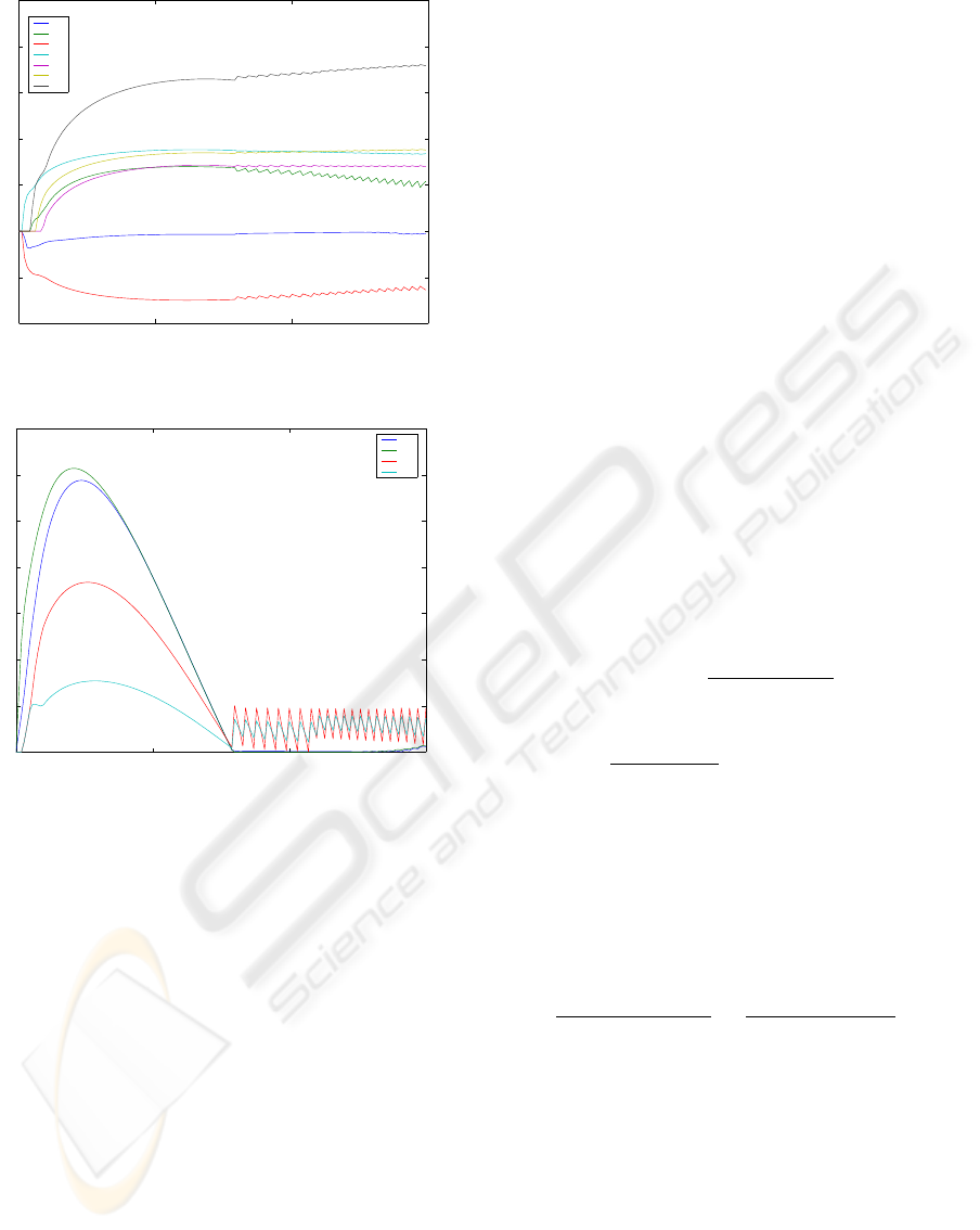
6.2 Algorithm performance

Performance with dynamical source rates is shown

in ﬁgures 7 and 8. The bundle algorithm with con-

stant step sizes α = 2.5 and β = 0.2 performs very

well. We note that it dynamically adjusts link ﬂows

(t) as the network load changes. We notice that

during the time when network is over-saturated, the

queue lengths grow; however, as soon as user trafﬁc

becomes feasible again, the queues are again driven

to zero.

Figures 9 and 10 show algorithm performance with

a more aggressive β parameter. We set constant step

sizes α = 2.5 and β = 1; therefore, we place more

weight on having small queue sizes. It is clear that

average queue size in the system is much smaller.

However, as we use larger step sizes our system be-

comes less stable. There is a clear trade-off between

queue size regulation and algorithm convergence and

smoothness.

DYNAMIC ROUTING AND QUEUE MANAGEMENT VIA BUNDLE SUBGRADIENT METHODS

0 50 100 150 200 250

−0.5

0.5

Figure 7: Flows x

(t) vs t with α = 2.5 and β = 0.2.

0 50 100 150 200 250

Figure 8: Queues q

(t) vs t with α = 2.5 and β = 0.2.

7 CONCLUSION

Subgradient bundle methods are not a new idea; the-

oretical work in this area was started around 1975

by Lamarechal and Wolfe. Years of research cul-

minated in the development of an optimization algo-

rithm suite that is commonly referred to as the bundle

methods, and which is in wide use today for many

non-differentiable optimization problems.

In this paper we have derived a bundle-like subgra-

dient method, which is completely distributed since it

uses only locally available network information, and

which simultaneously routes the network trafﬁc in a

dynamic manner and regulates queue sizes across the

network. Thus, we have achieved our goal of ﬁnding

a distributed algorithm for joint dynamic routing and

queue management. We are speculating that this is

the ﬁrst time that bundle subgradient ideas have been

applied to the network routing and the solution of the

optimal network ﬂow dual problem.

0 50 100 150 200 250

−0.5

0.5

Figure 9: Flows x

(t) vs t with α = 2.5 and β = 1.

0 50 100 150 200 250

Figure 10: Queues q

(t) vs t with α = 2.5 and β = 1.

We have proved the convergence of our proposed

algorithm and stated convergence conditions for con-

stant step size update rules. Algorithm performance

and theoretical results were successfully veriﬁed us-

ing Matlab simulations.

In the future, we would like to extend our algorithm

to the changing step size rules such as the diminish-

ing step size, and try to obtain absolute performance

limits for a bundle-type subgradient network routing

algorithm. We would also like to unify our sugradient

convergence proof method with works by (Athuraliya

and Low, 2000) and (Imer and Basar, 2003).

REFERENCES

Athuraliya, S. and Low, S. (2000). Optimization ﬂow

control – II: Implementation. http://netlab.

caltech.edu.

ICINCO 2004 - INTELLIGENT CONTROL SYSTEMS AND OPTIMIZATION

Bertsekas, D. P. (1999). Nonlinear Programming. Athena

Scientiﬁc, second edition.

Bertsekas, D. P. and Gallager, R. (1991). Data Networks.

Prentice-Hall, second edition.

Boyd, S. and Vandenberghe, L. (2003). Convex Optimiza-

tion. Cambridge University Press.

Boyd, S., Xiao, L., and Mutapcic, A. (2003). Subgra-

dient methods - EE392o class notes, Stanford Uni-

versity. http://www.stanford.edu/class/

ee392o/subgrad method.pdf.

Imer, O. and Basar, T. (2003). Dynamic optimization ﬂow

control. In IEEE Conference on Decision and Control,

pages 2082–2087.

Lamarechal and Wolfe (1975). Nondifferentiable optimiza-

tion. In Mathematical Programming Study, volume 3.

Segall, A. (1977). The modeling of adaptive routing in

data-communication networks. IEEE Transactions on

Communications, 25(1):85–95.

DYNAMIC ROUTING AND QUEUE MANAGEMENT VIA BUNDLE SUBGRADIENT METHODS

REFERENCES

Athuraliya, S. and Low, S. (2000). Optimization flow