THE EFFECTS OF INTERELEMENT SPACING IN LINEAR

ARRAYS ON THROUGHPUT PERFORMANCE IN AD HOC

NETWORKS

Sonia Furman, David E. Hammers, and Mario Gerla

Electrical Engineering and Computer Science Departments, University of California, Los Angeles

Los Angeles, California 90095, U.S.A.

Keywords: Ad hoc networks, Sidelobes, Fading, Hidden nodes, Directional antennas, QualNet

Abstract: With the high demand for improved signal link quality in ad hoc networks, devices configured with

omnidirectional antennas can no longer meet the growing needs in throughput performance, and alternative

approaches using antenna arrays that provide directional radiation patterns are sought. This study models an

8-element linear antenna array and examines the effects of interelement spacing of the array on the ad hoc

network’s throughput performance. We show through simulation, that as a result of the antenna array, the

throughput performance of the network consistently improved compared to that with an omnidirectional

antenna. Interestingly, we determined that the maximum increase in performance of over 150% was attained

with the smallest interelement spacing of

5.0

rather than with the larger interelement spacing and higher

gain. With null-steering, this performance increased even further to 180%.

1 INTRODUCTION

Attributes of ad hoc networks provide a powerful

combination of both mobile access and

configuration flexibility that enables fast deployment

critical to military applications and recovery

operations. Unlike cellular and radar communication

systems, ad hoc networks are local area networks

(LANs) that communicate over a medium with no

observable boundaries, are formed without pre-

planning, and exist only for as long as they are

needed (IEEE 1999). The inherent features that

make these networks so attractive are also those that

bring a higher level of complexity to the design of

protocols and transceivers. Although solutions to

enhance link quality using antenna arrays have been

employed extensively in other wireless

communication systems, this approach has not yet

been fully exploited in ad hoc networks and is still in

its infancy stages. To employ antenna arrays in

future devices associated with ad hoc networks,

challenges concerning the physical (PHY) and

medium access control (MAC) layers of the network

need to be addressed. These challenges include

modifying existing protocols associated with the

IEEE 802.11 standards (IEEE 1999, 2000) that will

accommodate effective beam steering policies, and

designing accurate antenna array models that reflect

realistic wireless channel conditions. Previous

studies (Ko, Shankarkumar & Vaidyn 2000;

Nasipuri el al. 2000; Ramanathan 2001), have

shown the benefits of directional antennas (antenna

arrays) in ad hoc networks by modifying MAC

protocols that provide effective mechanisms for

beam steering policies while using hypothetical

antenna models on both the transmitter and receiver.

This work like prior work, establishes the benefits of

antenna arrays in an ad hoc networks, yet differs

considerably from prior work in that it provides the

design of accurate antenna array models employed

only at the receiver, and determines through

simulation the effects of interelement spacing of the

array on the network’s throughput performance.

In the remainder of this paper, Section 2

presents a summary on the benefits of directional

antennas in ad hoc networks and discusses the

implications on the hidden node problem. Section 3

describes the design of the linear antenna array with

the three variants of interelement spacing. Section 4

discusses an analytical approach to maximize the

SINR in a fading channel. Section 5 provides the ad

hoc network environment used in the simulation and

150

Furman S., E. Hammers D. and Gerla M. (2004).

THE EFFECTS OF INTERELEMENT SPACING IN LINEAR ARRAYS ON THROUGHPUT PERFORMANCE IN AD HOC NETWORKS.

In Proceedings of the First International Conference on E-Business and Telecommunication Networks, pages 150-159

DOI: 10.5220/0001390701500159

 SciTePress

the results obtained, followed by a summary with

conclusions on the study in Section 6.

2 BENEFITS OF ANTENNA

ARRAYS IN AD HOC

NETWORKS

Benefits of antennas arrays in wireless ad hoc

networks have gained much interest in recent years

due to their potential to enhance network

performance. In comparison to an omnidirectional

antenna which produces an azimuthal radiation

pattern of 360

, the array produces a narrow beam in

which the confined energy (or main lobe) is pointed

in the direction of the desired signal resulting in a

notable reduction in interference, and the ability to

mitigate multipath, leading to improved channel

capacity and spectrum efficiency. Channel capacity

is a measure that describes the maximum data rate in

a channel of designated bandwidth (Blogh & Hanzo

2002), and improved channel capacity (or spectrum

efficiency) implies the support of more users within

that bandwidth without loss of throughput

performance. Omnidirectional antennas are among

the primary contributors to limiting channel capacity

and spectrum efficiency in ad hoc networks, thereby

creating a need for researchers to identify alternative

solutions and new approaches in the design of the

PHY layer.

Researchers suggest that there are substantial

performance improvements in throughput and packet

delay to be gained by employing directional

antennas in ad hoc networks. Ko, Shankarkumar,

and Vaidyn (2000) have shown that the bandwidth

efficiency and throughput performance increased

with an abstract directional antenna due to their

design of a medium access control protocol D-MAC.

Nasipuri et al (2000) also proposed a modified MAC

protocol to control a hypothetical 4-directional

antenna model at both the transmitter and receiver

for which the average throughput in the network

increased by 2 to 3 times compared to that with an

omnidirectional antenna. In a comprehensive study

on the performance of ad hoc networks with

approximate antenna patterns, results in throughput

improvement of 28-118% depending on network

density have been reported (Ramanathan 2001). A

72% throughput improvement has been documented

in (Sanchez, Giles &. Zander 2001) by utilizing 60

beamwidth antennas in an ad hoc network using a

specific beam selection policy. These observations

for the most part relied on modified MAC protocols

that provided additional attributes to accommodate

beamsteering routines for systems that incorporate

abstract antenna arrays, at both the transmitter and

receiver (Ko, Shankarkumar & Vaidyn 2000;

Nasipuri el al. 2000). In our work it was not

necessary to modify the MAC protocol but instead

we relied on the simulators ability to steer the beam.

From our array model, 24 beams were generated

(eight beams per each of the 3 variants of

interelement spacing), and tabulated in terms of gain

per 1

increments (through 360

), to perform the

simulation in all the scenarios.

A unique characteristics that continues to

perplex researchers in ad hoc networks, is that of the

hidden node problem. Of particular interest is the

effect of antenna arrays on the spectrum efficiency

of the network, subject to the hidden node problem.

The hidden node (terminal) problem has been known

to have an adverse effect on ad hoc networks

performance primarily due to access restrictions

inherent in the IEEE 802.11 MAC protocol

(Khurana, Kahol & Jayasumana 1998; Hadzi-

Velkove & Gavrilovska, 1999), where it is assumed

to be configured with an omnidirectional antenna.

The inefficiencies in communications that arise due

to the hidden node problem, and the potential

increase in performance attributed to the antenna

array are described below.

The scenario in which the hidden node problem

arises is when a transmitter outside the radio range

of a transmitting node is not aware of its neighboring

node receiving, and attempts to transmit, causing

interference or a garbled message. Peterson and

Davie (2000) define the hidden node problem as a

“…situation that occurs on a wireless network where

two nodes are sending to a common destination, but

are unaware that the other exists”. Figures 1(a)

through 1(d) attempts to capture the hidden node

problem with an omnidirectional antenna. The

circles represent the radio range of the nodes A, B, C

and D. We assume that all nodes have equal radio

range. In Figure 1(a), we assume that nodes A & C

attempt to send a message to node B at about the

same time. Node C does not know that A is

attempting to send to node B since A is hidden from

node C (C is out of radio range with A – ‘dashed

line’), and therefore a situation of collision arises.

THE EFFECTS OF INTERELEMENT SPACING IN LINEAR ARRAYS ON THROUGHPUT PERFORMANCE IN AD

HOC NETWORKS

151

(

)

(

)

C A

B D

(

)

C A

(

)

Figure 1: Hidden node problem with

omnidirectional antenna

This collision occurred in spite of the MAC

protocol designed to send and receive short control

frames, Ready-To-Send/Clear-To-

Send/Acknowledge (RTS/CTS/ACK), to ensure

collision avoidance in the multiaccess scheme

Carrier Sense Multiple Access with Collision

Avoidance (CSMA/CA). In Figure 1(b), both A & C

are attempting to connect to B at slightly different

times. Node A succeeds in establishing

communication with B, thereby blocking C from

transmitting or receiving. Note that this time only

the A circle is filled since it is the only node

transmitting, and since C is blocked it remains quiet

for the duration of the transmission between A & B.

In Figure 1(c), node D wants to send information to

C since it cannot detect that the channel is busy, i.e.

B is not within radio range of D (broken line

between B and D). Potentially, D may transmit but

not to node C because C is blocked on behalf of B

that is receiving from node A (B is within radio

range of C). In Figure 1(d), node D unnecessarily

has to wait to transmit to C at least until node A

completes its transmission to B, which clearly is

inefficient and undesirable. These inefficiencies

have been quantified in various studies (Khurana,

Kahol & Jayasumana 1998; Hadzi-Velkove &

Gavrilovska, 1999). Moreover, it has been shown

that the throughput consistently declined as the

probability of hidden nodes increased (Hadzi-

Velkove & Gavrilovska 1999). Khurana, Kahol &

Jayasumana (1998) have shown through simulation

that throughput is acceptable when the number of

hidden pairs is less than 10%, but then degrades

significantly when the number of hidden pairs

increases.

Figure 2 suggests that by using an antenna array

in the above network access scenarios, the

throughput will increase significantly. In Figure 2,

nodes A & B perform the RTS\CTS\ACK

handshake, using omnidirectional communication.

B goes into the receive data mode with a directional

antenna pointed at A. We repeat the scenario for

Figure 1(c) where D wants to transmit to C. In this

case, once B is in the receive mode, C is no longer

blocked to receive, and D may transmit to C as long

as B is receiving from A but not transmitting to A.

Node C, using a directional beam may now receive

from D without creating interference to B even

though C is in radio range of B. Using directional

beams in the network, the 2 additional nodes (C &

D) which otherwise may have been blocked, or have

been in a wait mode like node D in Figure 1(d) are

now able to communicate compared to only 2 nodes

communicating in Figure 1. This example clearly

demonstrates the potential of an antenna array to

increase network capacity and spectrum efficiency

in an ad hoc network.

3 SYNTHESIS OF THE LINEAR

ARRAY

Antenna synthesis in its simplest form is a methodic

process whereby a radiation pattern defined in terms

of its main beam and sidelobes is obtained from a

specific antenna configuration in which the

hardware design constraints (current, coupling, etc.)

of the antenna are satisfied. Figure 3 summarizes

the parameters associated with antenna synthesis.

Synthesis methods for the most part rely on the

relationship between the excitation current of the

array and the pattern generated.

Figure 2: Increased network capacity with

directed beams from antenna array

B D

ICETE 2004 - WIRELESS COMMUNICATION SYSTEMS AND NETWORKS

152

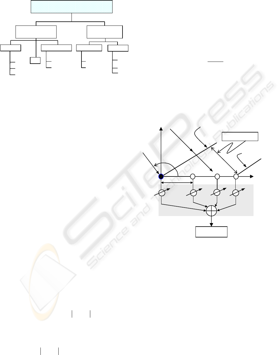
Figure 4: Linear array - UE ESLA

-1 m 1

In our design, we used these parameters as a

guide to generate radiation patterns for narrow main

beams and low sidelobes with an antenna type of a

linear array shape (Figure 4). The desired

normalized radiation pattern F(

) of a linear array

with parallel uncoupled elements (along the x-axis)

is defined in (1) as the product of the element pattern

of the array g

(

), and the array factor f(

)

(Stutzman & Thiele 1998).

Output

plane wave

front incident

on element

wave

ment

incident on

ele

θφ

sincosdd =∆

(

)

1−M

Fgf

(,) (,) (,)

(1)

where:

and

are the elevation and azimuthal angle

respectively of the plane wave impinged on the

array.

The directional properties of the radiation

pattern are usually described by the power pattern,

which originates in the Poynting vector S measured

in Watts/m

, that gives the angular dependence of

power on the variation of (

) of the originating

radiation source. The instantaneous value of S

describes the magnitude and direction of the

power/m

that is parallel to the xy plane, and is

derived from the cross product of the electric field

density (E), and the complex conjugate magnetic

field (H*) vectors, expressed in V/m and A/m units

respectively. The direction then of S (or the power)

is perpendicular to the xy plane (E

plane).

Hence, for z-directed sources the normalized power

pattern is (2).

),(),(

φθφθ

FP = (2)

It could be easily shown that when the radiation

pattern F(

) is expressed in volts, (not

normalized), then the power expressed in dB units is

the same as the radiation pattern in dB. i.e.

FP ),(),(

φθφθ

= . The radiated power ),(

of the beam in (3) is related to the antenna

directivity G

(,)

in (4) by means of the power

density

Antenna Synthesis

)

which is the power per unit solid

angle in the direction (

) expressed in

Watts/(rad)

φθθφθφθ

ddUP

∫∫

sin),(),( (3)

avg

(,)

θφ η

(4)

where:

is the antenna efficiency factor, and U

avg

the average power density

4/),(P of an

isotropic antenna. The antenna gain is then

expressed in dBi rather than in dB. For the ideal case

where there are no losses at the antenna and perfect

impedance matching,

=1 and the expression in (4)

is termed the gain, i.e. the gain is related to the

directivity of the antenna only by the efficiency

factor

. In our model, we assume,

=1 and that

gain and directivity are interchangeable.

Though we used the antenna synthesis

parameters to derive at the radiation patterns, we

chose not to use the Dolph-Chebyshev synthesis

method that deals with low sidelobes and narrow

main beam design, since the solution to those

polynomials depend only on the number of elements

in the array and not on the interelement spacing,

which is pivotal to the array design in this work.

Figure 3: Antenna synthesis parameters

Continuous

Discrete

Continuit

Sha

Linear

Planar

Conformal

Size

Main bea

arrow

Shaped

Parameters fo

antenna type

Radiation pattern

Sidelobe

ominal

Low

Shaped

THE EFFECTS OF INTERELEMENT SPACING IN LINEAR ARRAYS ON THROUGHPUT PERFORMANCE IN AD

HOC NETWORKS

153

We designed a linear equally spaced antenna

array, consisting of 8 elements along the x-axis with

interelement spacing d as shown in Figure 4. We

assumed the elements of the array to be identical,

uniformly excited (UE), and that the array factor

) represents the sum over the currents for each

element weighted by the spatial phase delay

from each element to the far-field point (Stutzman &

Thiele 1998). The UE equally spaced linear array

(ESLA) in Figure 4 attempts to capture Figure 3-3

from Liberti & Rappaport (1999, Pg 85) that

describes the basis for the design used in this work.

As shown in Figure 4, the impinged plane wave

arriving from an angle (

) relative to the x-axis

will travel an additional distance

before arriving at element m,

relative to the element at the origin. The difference

in phase

θφ

sincosdd =∆

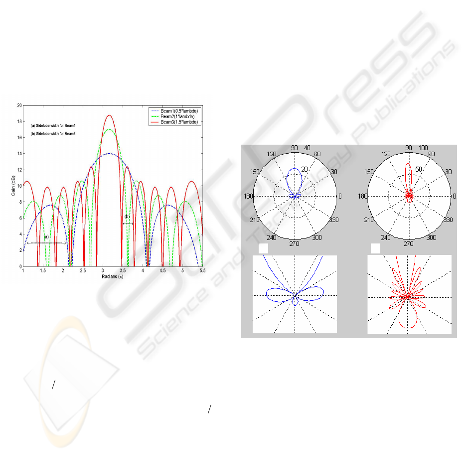
(a) (b)

Figure 6: Polar representation of patterns for

interelement spacing (a) d1 (b) d3

∆

between the signal component on

element m and the element at the origin is (5).

cossinsinsincos(

mmmm

zyxd +

=∆=∆

(5)

where:

is the phase propagation factor and is

equal to

Assuming the elevation angle

is equal to

and substituting

in (5), the received signal

at antenna element m along the x-axis is (6)

without taking noise/interference into consideration,

and the output of the array z(t) is (7). In vector

notation the left side of (7) is represented in (8).

dmx ∆=

)(tx

θφβ

sincos

)(

)()(

mdj

dmj

etAs

tstx

−

∆−

(6)

),()()()()(

sincos

φθ

θφβ

ftAsewtAstxwtz

mdj

mmm

===

−

∑∑

(7)

where: A is an arbitrary gain constant, s(t) is the

baseband complex envelope representing the

modulation of the plane wave,

),(

is the array

factor, and

the weighting element associated

with the m

branch of the array where

φβ

cosmdj

ew =

xwz

(8)

where:

121,0 −M

110 M

−

and H, the Hermitian operator is the complex

conjugate (*) of the transpose vector

],...,,[= xxxxx )],,,([

www= Kw

The UE-ESLA used in the design for this study

represents three configurations based on

interelement spacing:

5.01 =d

12 =d

, and

5.13

, corresponding to Beam1, Beam2, and

Beam3 respectively in Figure 5, which shows the

gain as a function of the interelement spacing. By

adjusting the set of weights

, it is possible to

direct the boresight (the direction of maximum

radiated power in the main beam) of the array

pattern in any desired direction of

. As shown

in Figure 5, Beam1 represented by the antenna

pattern with an interelement spacing

5.01 =d

, has a

boresight of 14.024dBi. Beam2 (green) -

, a

Figure 5: Linear array with three variants on the

interelement spacing

ICETE 2004 - WIRELESS COMMUNICATION SYSTEMS AND NETWORKS

154

boresight of 17.013dBi, and Beam3 (red) where

5.13 =d

has the maximum gain in its boresight of

18.774dBi. It is readily seen in Figure 5 that the

larger the interelement spacing, the higher the gain

and sidelobe peaks. Thus for d3, the gain of the

main beam pattern (boresight) and its sidelobes are

the highest (Figure 5(b)), while for d1, the gain of

the main lobe and its sidelobes are the lowest

(Figure 5(a)). To quantify the beam width we used

the metric Half Power Beamwidth (HPBW), which

describes the angular width between the points on

the main lobe that are 3dB below the boresight. The

HPBWs for Beam1, 2 and 3 are 106

, 52

, 34

respectively. Another metric of interest that

describes the characteristics of the radiation pattern

is the sidelobe level (SLL) and is defined as the ratio

between the absolute maximum value of the largest

sidelobe to the absolute maximum value of the main

lobe (Stutzman & Thiele 1998).

It is readily seen that as the interelement spacing

increases the HPBW decreases, and the sidelobe

peak increases. This will have profound implications

on the throughput performance, as we will see later

in Section 5. It is interesting to note that the SLL for

all three interelement spacing is nearly the same (in

the vicinity of minus 12.8dB) in spite of the fact that

the sidelobe peak of Beam1 (Figure5) is

significantly less than that of Beam3. Therefore, one

may assume that Beam3 would be more vulnerable

to interference than Beam1 although the SLL for

both beams is the same. This fact is more

pronounced in Figure 6. Both Figures 6a and 6b are

the polar representations of Beam1 and Beam3

respectively with an enlargement view of their

sidelobes immediately below. We distinctly see that

as the interelement spacing increased the number of

sidelobes increased, and the gain of the backlobe

(Figure 6b) increased significantly, presenting a

higher risk with respect to interference. The extra

main lobes formed with large interelement spacing

are referred to as grating lobes.

4 MAXIMIZING THE SINR IN

FADING CHANNELS

The mobile radio channel in ad hoc networks

deviates considerably from the stationary additive

white Gaussian noise (AWGN) channel due to

continuous variations in the environment, motion of

surrounding objects, and the mobility of the device

itself. In such an environment, the transmitted signal

arrives at the receiver from different paths

(multipath) caused by its wave scattering off of

building and objects, which results in delays and

attenuation of the received signal at the antenna

elements. This phenomenon known as fading is used

in wireless communication to describe the

fluctuation in the amplitude and phase of a radio

signal over a time period or travel distance. Fading

can lead to significant degradation in the reception

of the desired signal or in the signal to noise plus

interference ratio SINR, resulting in unacceptable

levels of throughput in the network. In non-

frequency selective fading (or flat fading) channels

where the signal bandwidth is less than the channel

bandwidth, variations in amplitude of the multipath

signals arriving at the receiver may be expressed

statistically in terms of a Rayleigh probability

distribution function. It has been shown (Furman,

Hammers & Gerla 2003) that with mobility the

signal strength of the envelope of the received signal

has deep fades that may dip as low as –10dB, which

is significantly below the threshold when compared

with the no-mobility case. These flat-fading results

may require up to 20 to 30dB more transmitter

power to acquire the equivalent bit error rate (BER)

performance of that obtained in an AWGN channel.

To meet the increased demand of SINR that will

result in increased throughput, directional antennas

may well be the solution as discussed in Section 2.

To maximize the SINR analytically in a fading

channel, we considered two basic configurations as a

function of interelement spacing. The first

configuration is associated with a fraction of a

wavelength interelement spacing (e.g.

)5.0

as in

Beam1, and is usually considered an adaptive array.

An adaptive array employs small (fractional

interelement spacing to avoid grating lobes and

relies on various algorithms (Monzingo

& Miller

1980) to dynamically adjust the weights

associated with each branch of the array in Figure 4.

Some of these algorithms may also be used to

generate optimum weights in fixed beam arrays,

consistent with the weights used in this work. The

second configuration assigns interelement spacing in

multiplies of

. This configuration corresponds to

Beam2 and Beam3 in our design, and is usually

referred to as ‘combining methods’ in antenna

diversity. In the second configuration, the weights

assigned to each of the branches are predefined.

THE EFFECTS OF INTERELEMENT SPACING IN LINEAR ARRAYS ON THROUGHPUT PERFORMANCE IN AD

HOC NETWORKS

155

To determine the optimum weight assignment that

will maximize the SINR in a fading channel, we first

expand on the description of the signal in (6) to

include the interference and noise

at each of

the antenna elements of the receiver (9).

)(tn

(9)

)()()( tntstx

mmm

The output z(t) of the array then comprises of

two components the desired signal z

, and the

noise/interference component z

(10), and is

represented in (11) vector form.

∑

−

mmn

mms

nwz

swz

(10)

(11)

where:

and

are

the desired signal and the noise associated with the

antenna elements respectively.

ssss ],[

1,,21,0 −

nnnn ],[

1,,21,0 −

The average noise power is then (12).

wRw

wNNwwNNw

THTH

EEzEP

=== ][][][

(12)

where:

is the correlation matrix of the noise

defined by

])()([

tntnE

The noise correlation matrix

for the 8-

element linear array is then (13), where (

•

)

represents convolution, and the bars above each

entry within the matrix represent average.

⎥

⎦

⎤

⎢

⎣

⎡

•••

)()()()()()(

882818

822212

82111

tntntntntntn

MLMM

(13)

The computation of R

in (13) is significantly

simplified by transforming the convolution in the

time domain into multiplication of the individual

transforms in the frequency domain. Similarly, an

expression for the average signal output power may

be expressed in (14).

wRw

P =

(14)

where:

is the correlation matrix (or the

covariance matrix with zero mean) of the desired

signal.

The cost function (15) then is defined as the

ratio of the average noise power to the average

(desired) signal power (14).

wRw

wJ =)( (15)

To minimize the cost function in (15), we take

the derivative of the numerator and set it to zero, i.e.

we use the gradient operator

on or

. As a sideline, it should be noted that

since the diagonal elements of the noise correlation

matrix in (13) are real, the matrix is Hermetian,

which implies that a matrix A exists for which

, where I is an identity matrix. This

matrix identity is essential in order to derive at the

solution for the cost-function in (15). The optimal

solution to minimizing (15) is (16) (Monzingo

Miller 1980).

∇

)( wRw

∇

IARA =

wwRR

max

−

(16)

where:

max

is the maximum eigenvalue of the

signal covariance matrix

. To find the

eigenvalues that satisfy (16) we expand the

determinant

IRR

−

Both configurations described in this section use

complex weights to adjust the incoming signal from

each antenna element, which are then combined

(summed) into a signal directed to the receiver’s

detector. For this study, we assumed that the weights

associated with each of the elements are fixed and

provide equal gain in all directions. The weights

derived to maximize the SINR were varied only as a

function of the interelement spacing d.

5 NETWORK SIMULATION AND

RESULTS

To perform the network simulation for this study we

used the QualNet simulator (SNT, 2002), which is a

discrete event high performance networking research

tool for various configurations of wired and wireless

networks. QualNet supports directional antennas and

ICETE 2004 - WIRELESS COMMUNICATION SYSTEMS AND NETWORKS

156

100 150 200 250

Throughput (Kbps)

omni

10 0 150 2 0 0 2 50

Throughput (Kbps)

100 150 200 250

Throughput (Kbps)

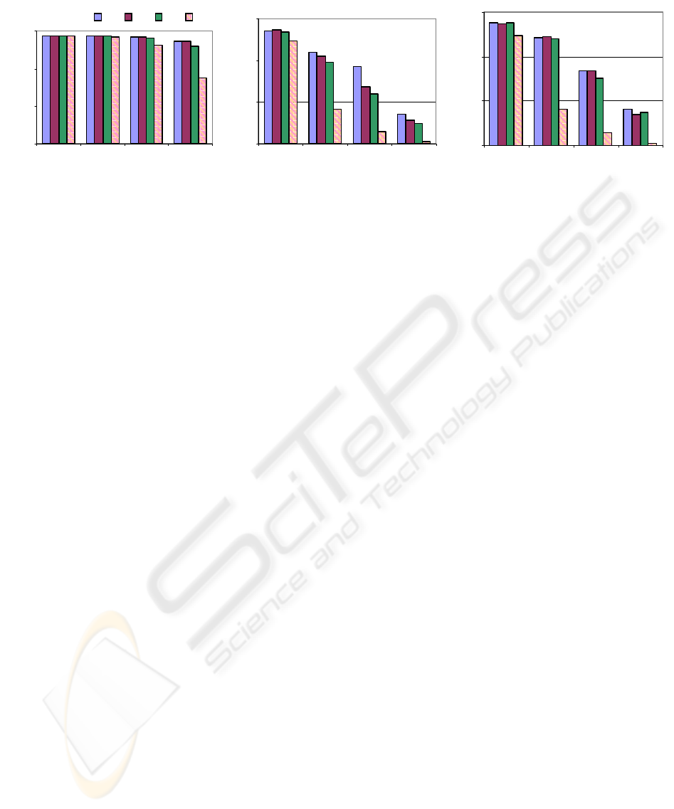
# of Nodes # of Nodes # of Nodes

(a) (b) (c)

Figure 7: Throughput performance as a function of network density (a) AWGN channel (b) Fading channel

has the built-in capability to steer the radiation

pattern of the antenna array in the direction of

communication.

The ad hoc network for the simulation was

based on the IEEE802.11b standard (IEEE, 2000),

and the environment for the simulation comprised of

a terrain 1600x1600m with 100, 150, 200, and 250

nodes randomly distributed. Experiments were

performed with the assumption that the nodes are

mobile, and we used the Random Waypoint mobility

algorithm to implement mobility (with speeds 0 to

10m/s, and 0 pause time). The ad hoc on-demand

vector distance (AODV) routing protocol was used

in all the scenarios of the simulation. We used

differential quadrature pulse shift keying (DQPSK)

modulation, which adjusts the carrier and bit timing

to produce the in-phase (I) and quadrature (Q)

components of the transmitted signal. The minimum

threshold for the receiver was set at -81dBm and its

sensitivity at -91.0dBm. The carrier frequency used

was f

=2.4GHz with a data payload of 2Mbps.

Traffic was generated using a constant bit rate

(CBR) generator with a ratio of 1:5 sessions per

CBR. Data transfer was at 4 packets/s and each

packet was set at 512 bytes in length. The results

obtained from the network simulation represent an

average of 5 runs with random seeds in the

configurations described above for each of the three

radiation patterns derived from the interelement

spacing, in reference to an omnidirectional antenna.

In addition, we repeated the entire set of simulation

described above with null-steering by suppressing

the sidelobes for each the three patterns. All the

simulation experiments were performed for both

AWGN and Rayleigh (fading) channels. The

distributed coordination function (DCF) of the IEEE

802.11 (IEEE, 1999) MAC protocol was used to

implement the CSMA/CA protocol. A refinement to

this access method implements RTS, to further

minimize collisions prior to data transmission. The

additional overhead however, of the RTS

mechanism may not always be justified (Gerla,

1997). Accordingly, the MAC protocol was

modified to disabled the RTS in order to reduce

bandwidth overhead.

Two scenarios, low-density and high-density are

presented (we define density as #nodes/area). The

low-density addresses the performance for 100-150

nodes, and the high-density for 200-250 nodes. The

results obtained from the simulation are shown in

Figure 7(a)-(c). For the AWGN channel (Figure

7(a)) the performance difference between the

omnidirectional antenna and the arrays in the low-

density case was less than 1% (on the average). In

the high-density case, the performance with the

arrays was at least 22% better than with the

omnidirectional antenna. For the fading scenario in

Figure 7(b), the performance difference between the

omnidirectional antenna and the arrays in the low-

density scenario increased significantly and was

computed to be 37% (compared to the 1% above),

and 152% (compared to the 22% above) for the

high-density. Figure 7(c) is an extension of the

simulation represented by Figure 7(b), with the

exception that in this case we used null-steering to

improve performance. With null steering, the

performance increased for all three variants of

interelement spacing. The performance improvement

in the fading channel with null-steering for the low-

density scenario was on the average 46%, where as

for high-density the improvement was

THE EFFECTS OF INTERELEMENT SPACING IN LINEAR ARRAYS ON THROUGHPUT PERFORMANCE IN AD

HOC NETWORKS

157

approximately 180% with respect to the

performance of an omnidirectional antenna.

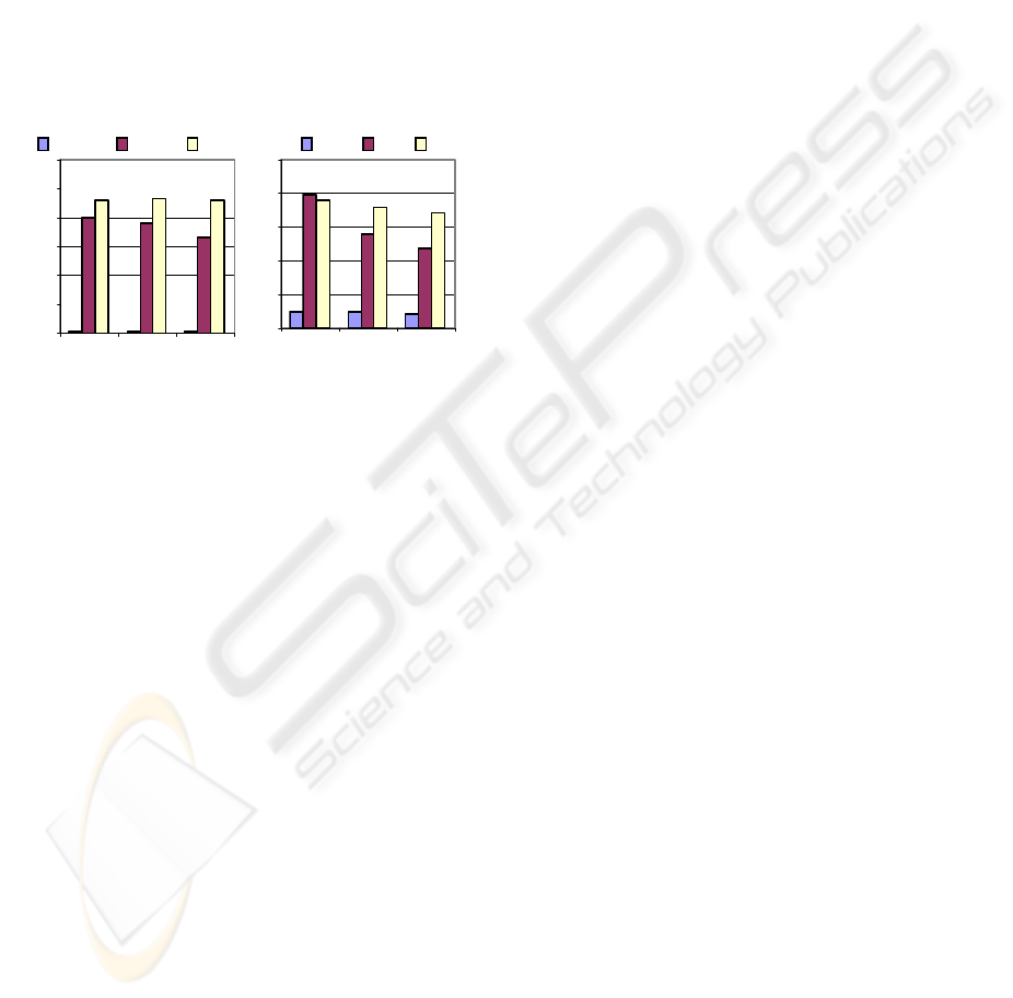
Figure 8 shows the relative performance as a

function of interelement spacing in both low and

high density for channel conditions with no fading -

‘nF’, with fading -‘F’, and with fading and null-

steering - ‘F_ns’. It is clearly seen from Figure 8,

that the d1 interelement spacing in all the

experiments attained the maximum performance.

This fact is interesting since the gain of the array

with d2 and d3 interelement spacing is greater than

that of d1 (Figure 5), yet the performance was less,

which is contrary to an intuitive prediction.

0.1

0.2

0.3

0.4

0.5

0.6

d1 d2 d3

Int erelement spaci ng

Improvement (%)

nF F F

0.5

1.5

2.5

d1 d2 d3

Int er el ement spaci ng

nF F F

(a)

Figure 8: The relative throughput performance

improvement as a function of interelement spacing

(a) Low density (b) High density

6 SUMMARY AND

CONCLUSIONS

In this work, we discussed the benefits of directional

antennas in ad hoc networks and the necessity to

supplement prior work with accurate directional

antenna design models. We used antenna synthesis

to guide the design of the antenna arrays, and in

Section 4 described an analytical approach to

determine the optimum weight

that maximizes

the SINR. The radiation patterns from the design of

the linear array with the three variants of

interelement spacing (d1, d2, and d3) were then used

in the network simulation to quantify the effects of

interelement spacing on throughput performance for

both low and high densities network scenarios. In

each scenario, we compared the throughput

performance in an AWGN channel, a fading channel

(Rayleigh fading), and finally in a fading channel

utilizing null-steering.

We conclude that regardless of the interelement

spacing in the linear array, the throughput

performance in the network increased compared to

that of an omnidirectional antenna. The effects of

the interelement spacing on the performance of the

network were not necessarily predictable, and were

in fact the case where ‘less is more’. The results

show that Beam1 (smallest interelement spacing d1)

with the lowest gain, interestingly performed the

best and resulted in a higher throughput

performance, while Beam3 (d3 interelement

spacing), with the most gain consistently produced

the lowest results. These results are attributed to (a)

the mobility of the nodes, and (b) amplification of

the interference in the sidelobes. As the beam

became narrower (more gain, larger interelement

spacing, and lower HPBW), the node due to

mobility drifted out of the main beam area faster

than with the wider beam, thereby producing inferior

results compared to that of the wider beam with

lower gain. Further, the amplification of interference

was greater as the interelement spacing increased

because the grating lobes increased and the peak of

the sidelobes increased, leaving Beam1 to perform

superior with respect to interference. Finally, we

conclude that in an AWGN channel the use of

antenna arrays were not meaningful in the low-

density network scenario while for a realistic

channel model (a Rayleigh channel), antenna arrays

can substantially increase network performance and

in some cases, the increase may be as high as 197%.

REFERENCES

Blogh J. S., and Hanzo, L., 2002. Third Generation

Systems and Intelligent Wireless Networking, John

Wiley & Sons, Ltd, New York.

Furman, S., Hammers, D. E., and Gerla, M., 2003.

“Optimum Combining for Rapidly Fading Channels in

Ad Hoc Networks”, SCI’03 Proc. of The 7

World

Multiconference on Systemics, Cybernetics and

Informatics vol. III, July 27-30, Orlando, pp 49-54.

Gerla, M. and Talucci, F., 1997. “MACA-BI (MACA By

Invitation) A Wireless MAC Protocol for High Speed

ad hoc Networking”, Universal Personal

Communication Records, IEEE, 6

International

Conference, vol. 2, pp. 913-917.

Hadzi-Velkov, Z., and Gavrilovska, L., 1999. “Influence

of Burst Noise Channel and Hidden Terminals over

the IEEE 802.11 Wireless LANs”, VTS’99, Vehicular

ICETE 2004 - WIRELESS COMMUNICATION SYSTEMS AND NETWORKS

158

Technology Conference, IEEE, 50

Conference, vol.5,

pp. 2641-2945.

IEEE Std. 802.11, 1999. “Wireless LAN Medium Access

Control (MAC) and Physical Layer (PHY)

Specifications”, The Institute of Electrical and

Electronics Engineers, Inc., ISBN 0-7381-1658-0.

IEEE Std. 802.11b-1999, 2000. “Wireless LAN Medium

Access Control (MAC) and Physical Layer (PHY)

Specifications: Higher-Speed Physical Layer

Extension in the 2.4 GHz Band”, The Institute of

Electrical and Electronics Engineers, Inc., ISBN 0-

7381-1811-7.

Khurana, S., Kahol, A., and Jayasumana, A. P., 1998.

“Effect of Hidden Terminals on the Performance of

IEEE 802.11 MAC Protocol”, LCN’98, Local

Computer Networks Proc. 23

, pp. 12-20.

Ko, Y-B., Shankarkumar, V., and Vaidyn, N.H., 2000.

“Medium Access Control Protocols using Directional

Antennas in Ad Hoc Networks”, IEEE INFOCOM, pp

13-21.

Liberty, J.C. Jr., and Rappaport, T.S., 1999. Smart

Antennas for Wireless Communications: IS-95 and

Third Generation CDMA Applications, Prentice Hall,

Upper Saddle River, NJ.

Monzingo, R.A., and Miller, T.W., 1980. Introduction to

Adaptive Arrays, John Wiley & Sons, New York.

Nasipuri, A., et al, 2000. “A MAC Protocol for Mobile Ad

Hoc Networks Using Directional Antennas”,

WCNC’00,Wireless Communications and Networking

Conference, IEEE, vol.3, pp. 1214-1219.

Peterson, L. L., and Davie, B. S., 2000. Computer

Networks A Systems Approach, Morgan Kaufmann

Publishers, 2

edition, San Francisco.

Ramanathan, R., 2001. “On the performance of Ad Hoc

Networks with Beamforming Antennas”,

MOBIHOC’01, International Symposium on Mobile

Ad Hoc Networking & Computing, Proc. ACM, pp.

95-105.

Sanchez, M., Giles, T., and Zander, J., 2001.ACSMA/CA

with Beam Forming Antennas in Multi-hop Packet

Radio@, Radio Communication Systems, Proc. of the

Swedish Workshop on Wireless Ad-hoc Networks.

SNT, 2002. “QualNet Simulator & User’s Manual”,

Scalable Network Technologies, Inc., Los Angeles.

Stutzman, W. L., and Thiele, G. A., 1998. Antenna Theory

and Design, John Wiley & Sons, Inc., 2

edition, NY.

THE EFFECTS OF INTERELEMENT SPACING IN LINEAR ARRAYS ON THROUGHPUT PERFORMANCE IN AD

HOC NETWORKS

159