PACKET SCHEDULING ALGORITHM WITH WEIGHT

OPTIMIZATION

Ari Viinikainen, Jyrki Joutsensalo, Mikko P

akk

onen and Timo H

ainen

Department of Mathematical Information Technology, University of Jyv

askyl

P.O. Box 35 (Agora)

40014 University of Jyv

askyl

a, FINLAND

Keywords:

Packet scheduling, ﬂat pricing, revenue maximization, quality of service (QoS).

Abstract:

In this paper we present a scheduling algorithm for trafﬁc allocation. In our model, we use a ﬂat pricing sce-

nario in which the weights of the queues are updated using revenue as a target function. Due to the algorithm’s

closed form nature, it is capable of operating in non-stationary environments. In addition, the algorithm is

nonparametric and deterministic in the sense that any assumptions about the call density functions or duration

distributions are not made.

1 INTRODUCTION

Numerous pricing proposals have been developed for

the efﬁcient use of packet–switched networks. Here,

we review the research work that has similar features

as in our model. Several researchers have proposed

a pricing approach in which a small number of ser-

vice classes (between 2 and 4) should be offered on

the network in order to achieve service differentiation

(Gubta et al., 1997; Odlyzko, 1999; Gibbens et al.,

2000).

The pricing of a single network which provides

multiple services at different performance levels is

studied in (Cocchi et al., 1993). They present a good

example which shows that in comparison to ﬂat rate

pricing for all services, a price schedule based on

performance objectives can enable every customer to

derive a higher surplus from the service, and at the

same time, generate a bigger revenue for the service

provider. Reference (Gibbens and Kelly, 1999) de-

scribes yet another scheme for packet-based pricing

as an incentive for more efﬁcient ﬂow control.

However, it seems that packet-based pricing

schemes are not always appropriate, because real-

time trafﬁc requires QoS (Quality of Service) mea-

sures that are hard to analyze (Kelly, 1996; Bertsi-

mas et al., 1998b; Bertsimas et al., 1998a; Paschalidis,

1999).

The pricing of multiple services in single net-

work, with guaranteed QoS requirements, is studied

in (Keon and Anandalingam, 2003), where the opti-

mal pricing problem is formulated as a nonlinear in-

teger expected revenue optimization problem.

A static pricing schedule, based on dynamic pro-

gramming is proposed in (Paschalidis and Tsitsiklis,

2000) for maximization of the revenue and social wel-

fare and is extended to multiple service loss networks

in (Paschalidis and Liu, 2002).

Our research differs from the above studies by link-

ing pricing and queuing issues together; in addition,

our model does not need any excess information about

user behavior, utility functions etc. (as most pricing

and game-theoretic approaches do). This paper ex-

tends our previous pricing and QoS research (Jout-

sensalo et al., 2003a; Joutsensalo et al., 2003b; Jout-

sensalo et al., tion), where linear pricing algorithm

has been investigated. However, the ﬂat pricing algo-

rithm seems more realistic and is now the scope of our

studies.

We consider pricing and scheduling issues to

manage multiple communications services in single

telecommunication network. Different services are

grouped into service classes, differing in resource re-

quirements and tolerating different quality limitations

such as loss of data and transmission delay. The

proposed ﬂat algorithm takes also into account the

variable average data packet sizes in different trafﬁc

classes. The QoS and revenue aware scheduling al-

gorithm is studied in a single node case. It is derived

from a Lagrangian optimization problem, and an op-

timal closed form solution is presented.

The rest of the paper is organized as follows. In

127

Viinikainen A., Joutsensalo J., Pääkkönen M. and Hämäläinen T. (2004).

PACKET SCHEDULING ALGORITHM WITH WEIGHT OPTIMIZATION.

In Proceedings of the First International Conference on E-Business and Telecommunication Networks, pages 127-133

DOI: 10.5220/0001390901270133

 SciTePress

Section 2, the proposed ﬂat pricing scenario is pre-

sented and generally deﬁned. A closed form schedul-

ing algorithm is also derived in this section. Section 3

contains experimental part justifying theorems. Con-

clusions are presented and discussions about the fu-

ture work is made in Section 4.

2 THE FLAT PRICING

SCENARIO AND ALGORITHM

The scheduling mechanism is one of the major com-

ponent for providing differentiated service levels. In

our scheduling model, the weights of the queues are

dynamically updated based on the QoS and pricing

criterions of the service classes. In other word, the

weights for different classes can be assigned in a way

that the performance of high priority classes is guar-

anteed and no starvation of low priority classes occur.

The pricing scenario consists of m different traf-

ﬁc classes for different applications and priorities. In

our scenario we have four classes, m = 4, which are

referred to as the platinum, gold, silver and bronze

classes (Table 1). The platinum and gold classes are

reserved for the realtime and the lower priority classes

(silver and bronze) for non–realtime purposes. As an

example of the four classes, Voice over IP (VoIP) and

video conference trafﬁc streams belong to the plat-

inum and gold classes, respectively. Video streams

(e.g. MPEG4) are considered as a silver class cus-

tomers and File Transfer Protocol (FTP) ﬂows be-

long to the lowest priority (bronze) service class. The

platinum class customers are willing to pay for some

guaranteed bandwidth, delay, jitter and packet loss

probability. The gold class customers are ready to pay

for guaranteed bandwidth, delay and delay variance

(jitter). The silver class customers are not so tight on

the QoS requirements. In the silver class bandwidth

and jitter should be guaranteed. In the bronze class

the guaranteed bandwidth and packet loss are the most

important QoS parameters, while the delay can vary a

lot.

Let us consider a packet scheduler which receives

packets to be delivered from m different queues (i.e.

classes). Now, let d

be the processing time of the

classiﬁer for transmitting data from one queue to the

output of a packet scheduler. The data packets have

variable sizes and the average packet size for class i

is E(b

), i = 1, . . . , m.

In our scheduling model, the real processing time

(delay) for class i in the packet scheduler is

E(b

)

, (1)

where w

(t) = w

, i = 1, . . . , m are weights allotted

for each class, N

(t) = N

is the number of customers

and E(b

)(t) = E(b

) is the average data packet size

in the ith queue. Here, the time index t has been

dropped for convenience until otherwise stated and d

can be scaled to d

= 1 without loss of generality.

The natural constraints for the weights are

> 0 (2)

and

i=1

= 1. (3)

Without loss of generality, only non-empty queues are

considered, and therefore w

6= 0, i = 1, . . . , m. If

some weight is w

= 1, then m = 1, the packet size

can be scaled to E(b

) = 1 and the only class to be

served has the minimum processing time d

= 1, if

= 1. For each service class, a pricing function

) = r

(

E(b

)

+ c

) (4)

(euros/minute) is non-increasing with respect to the

delay d

. Here c

(t) = c

includes insertion delay,

transmission delay etc., and it is assumed to be con-

stant.

In the ﬂat pricing scenario, the pricing function is

deﬁned via maximum delay for each class and queue

as a QoS parameter.

The Gain factor r

of class i is measured by money

paid by one customer to the service provider per unit

time, e.g. euros/minute. Hence, the pricing function

in (4) reduces to the piecewise ﬂat function

) = r

, (5)

under the constraint

E(b

)

≤ d

i,max

, i = 1, . . . , m, (6)

where d

i,max

are preselected maximum delays to be

guaranteed. When N

customers are in the class (or

in the queue) i, the revenue achieved from that class

= N

(7)

euros/minute. Therefore, the total price paid by the

customers in m classes is

F =

i=1

(8)

under the constraint that the pre-selected maximum

delays d

i,max

are not exceeded. By using Lagrangian

approach, the revenue can be presented in the form

F =

i=1

+ λ(1 −

i=1

), (9)

where

E(b

)

. (10)

ICETE 2004 - SECURITY AND RELIABILITY IN INFORMATION SYSTEMS AND NETWORKS

128

Table 1: QoS parameters for different trafﬁc classes.

Trafﬁc class Type bandwidth e-to-e delay packet loss jitter

Platinum VoIP x x x x

Gold Video conference (H.263) x x x

Silver Video stream (MPEG4) x x

Bronze FTP x x

From (9) and (10), the revenue can be presented as

F =

i=1

+ λ(1 −

i=1

E(b

)

), (11)

F =

i=1

E(b

)

+ λ(1 −

i=1

). (12)

Optimal weights are obtained from the ﬁrst derivative

∂F

∂w

E(b

)

− λ = 0. (13)

λ =

E(b

)

E(b

)

E(b

)

(14)

(15)

Because

= 1, then

. (16)

From (10) and (16) one obtains

E(b

)

l=1

(17)

Equation (16) expresses the closed form solution to

the weights. Interpretation of (16) is obvious:

• Larger the gain factor r

is, larger is the correspond-

ing weight w

• Larger the number of users N

is, larger is the cor-

responding weight w

By using optimal weights, revenue F can be ex-

pressed as follows:

F =

i=1

E(b

)

i=1

E(b

)

i=1

E(b

)

i=1

E(b

)

, (18)

and F is

F =

i=1

E(b

)

(19)

with constraints

i=1

E(b

)

≤ 1, (20)

and

E(b

)

l=1

≤ d

i,max

, i = 1, . . . , m.

(21)

From (19) and (21) it is seen that gain factors r

, max-

imum allowed delays d

i,max

, as well as number of

users N

increase the revenue, which is a plausible

result. Also, as seen from (19), smaller packet sizes

increase the revenue.

Call Admission Control mechanism can be made

by simple hypothesis testing without assumptions

about call or dropping rates. Let the state at the time

t be N

(t), t = 1, . . . , m. Let the new hypothetical

state at the time t+1 be

(t+1), t = 1, . . . , m, when

one or several calls appear in some class/classes. In

hypothesis testing, revenue formula (19) is applied as

follows:

F (t) =

i=1

(t)

E(b

)

(22)

F (t + 1) =

i=1

(t + 1)

E(b

)

(23)

(t) =

E(b

)

l=1

(t) (24)

(t + 1) =

E(b

)

l=1

(t + 1) (25)

If F (t) >

F (t + 1) or maximum delay is exceeded

(

(t + 1) > d

i,max

), then call is rejected, otherwise

it is accepted.

3 EXPERIMENTS

The experiments demonstrate by simulation the ef-

fects of the maximum delays d

i,max

on the revenue.

In the experiments, calls and durations are Poisson

PACKET SCHEDULING ALGORITHM WITH WEIGHT OPTIMIZATION

129

and exponentially distributed, respectively. In addi-

tion, the number of classes is m = 4. The differ-

ent classes have different average data packet sizes

E(b

) = 1, E(b

) = 3, E(b

) = 5 and E(b

) = 10

kilobytes, with the platinum class (e.g delivering VoIP

trafﬁc) having the smallest size and the size increases

towards the bronze class (e.g delivering FTP trafﬁc).

Call rates per unit time for the platinum, gold, sil-

ver, and bronze classes are α

= 0.20, α

= 0.30,

= 0.40 and α

= 0.50, respectively. The dura-

tion parameters (i.e. ”decay rates”) are β

= 0.001,

= 0.003, β

= 0.005 and β

= 0.01, where prob-

ability density functions for duration are

(t) = β

−β

, , i = 1, 2, 3, 4 t ≥ 0. (26)

The number of unit times in the experiments was T =

2000.

Experiment 1. In the ﬁrst experiment, the four ser-

vice classes have the gain factors r

= 40, r

= 30,

= 20 and r

= 10. The maximum delays for the

classes are d

1,max

= 15, d

2,max

= 100, d

3,max

250 and d

4,max

= 1000. Fig. 1 shows the evolution

of the delays d

(t), d

(t) and d

(t) as well as

the maximum boundaries for them as a function of

time in the ﬁrst experiment. It is seen that the delays

are always below the maximum values, as guaranteed

by the constraint (21). Also, the delay boundary of the

platinum class is limiting the number of users in the

other classes as their delays are well beyond the limits

(i.e. the gold, silver and bronze classes could support

more users). Fig. 2 shows the number of users and

Fig. 3 the revenue in this experiment.

0 200 400 600 800 1000 1200 1400 1600 1800 2000

200

400

600

800

1000

1200

time

delays

Platinum

Bronze

Silver

Gold

Figure 1: Evolution of the delays d

(t) (platinum), d

(t)

(gold), d

(t) (silver) and d

(t) (bronze) as a function of

time in the ﬁrst experiment. The straight lines show the

maximum delays.

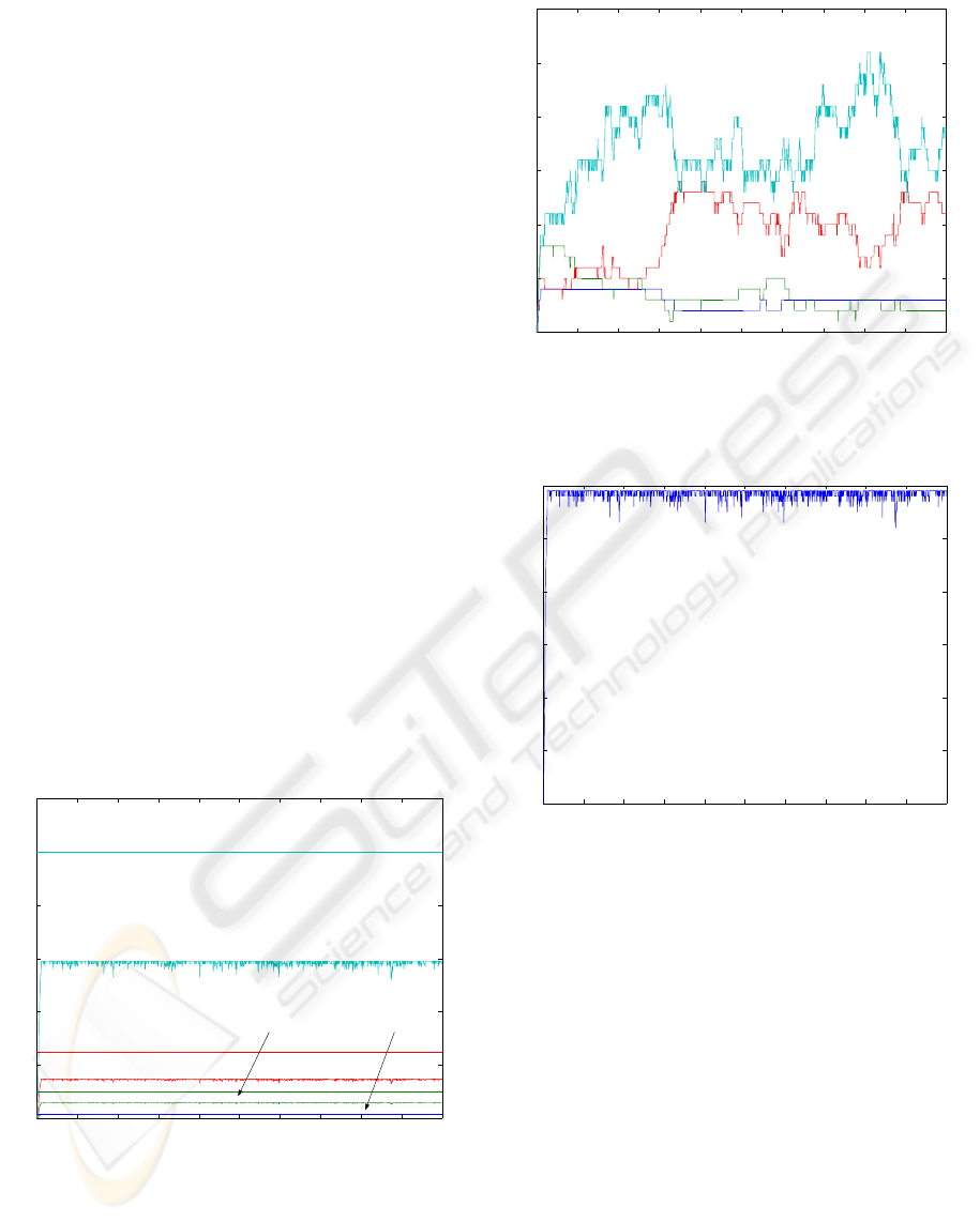
Experiment 2. In the second experiment, the pa-

rameters are as in experiment 1, except for the delay

of the platinum class, which is increased to d

1,max

0 200 400 600 800 1000 1200 1400 1600 1800 2000

time

number of users

Silver

Platinum

Gold

Bronze

Figure 2: Evolution of the number of users N

(t) (plat-

inum), N

(t) (gold), N

(t) (silver) and N

(t) (bronze) as

a function of time in the ﬁrst experiment.

0 200 400 600 800 1000 1200 1400 1600 1800 2000

100

200

300

400

500

600

time

revenue

Figure 3: Evolution of the revenue as a function of time in

the ﬁrst experiment.

25. By comparing Fig. 2 and Fig. 5 it is seen that

the number of users can be increased, while keeping

the delays below the deﬁned maximum values (Fig. 1

and Fig. 4). In Fig. 3 and Fig. 6 the increasing of

the revenue is due to the increase of the maximum de-

lay of the platinum class. This increases the number

of highly charged users more in the highest-priority

classes (Fig. 2 and Fig. 5) and decreases the overall

packet sizes in the queues, thus the revenue increases.

Experiment 3. In the third experiment we demon-

strate the effect of gain factors r

, by changing the

gain factor of the platinum class from r

= 40 to

= 100. The other parameters are the same as in

Experiment 1 (i.e. the platinum class delay boundary

is limiting the resources of the other classes). Now, by

comparing Fig. 1 and Fig. 7, it is seen that the delays

of the gold, silver and bronze classes are increased

ICETE 2004 - SECURITY AND RELIABILITY IN INFORMATION SYSTEMS AND NETWORKS

130

0 200 400 600 800 1000 1200 1400 1600 1800 2000

200

400

600

800

1000

1200

time

delays

Bronze

Silver

Gold

Platinum

Figure 4: Evolution of the delays d

(t) (platinum), d

(t)

(gold), d

(t) (silver) and d

(t) (bronze) as a function of

time in the second experiment. The straight lines show the

maximum delays.

0 200 400 600 800 1000 1200 1400 1600 1800 2000

time

number of users

Bronze

Gold

Platinum

Silver

Figure 5: Evolution of the number of users N

(t) (plat-

inum), N

(t) (gold), N

(t) (silver) and N

(t) (bronze) as

a function of time in the second experiment.

(but remaining under the constraints). This is due to

the fact that, now the number of users in the gold, sil-

ver and bronze classes is increased while the number

of users in the platinum class is decreased (Fig. 2 and

Fig. 8). In this case, by changing one of the gain fac-

tors, which lead to a different distribution of users in

the classes, the revenue is increased (Fig. 3 and Fig.

9).

These kinds of results give valuable information on

the tuning the model to work at the most optimal way

under different kind of trafﬁc scenarios e.g. at the

situations when the connection arrival rate varies at

different times scales - say night, morning, day, and

evening. This can also lead to the situation where the

customers of the highest trafﬁc classes move to use re-

0 200 400 600 800 1000 1200 1400 1600 1800 2000

100

200

300

400

500

600

700

800

900

1000

time

revenue

Figure 6: Evolution of the revenue as a function of time in

the second experiment.

0 200 400 600 800 1000 1200 1400 1600 1800 2000

200

400

600

800

1000

1200

time

delays

Bronze

Silver

Gold

Platinum

Figure 7: Evolution of the delays d

(t) (platinum), d

(t)

(gold), d

(t) (silver) and d

(t) (bronze) as a function of

time in the third experiment. The straight lines show the

maximum delays.

sources of the lower trafﬁc classes at night time. This

is because there is enough capacity available, and thus

needed QoS level can be achieved with the price of the

lower class.

Next, we present summary of our approach and the

experiments.

• The proposed weight updating algorithm is compu-

tationally inexpensive in our scope of study.

• The algorithm uses variable average data packet

sizes, taking into consideration the relative average

packet sizes in different classes.

• Experiments clearly justify the performance of the

algorithm, i.e. revenue curves are positive and the

delays remain below the predeﬁned limits.

• Some of the statistical and deterministic algorithms

PACKET SCHEDULING ALGORITHM WITH WEIGHT OPTIMIZATION

131

0 200 400 600 800 1000 1200 1400 1600 1800 2000

time

number of users

Bronze

Silver

Gold

Platinum

Figure 8: Evolution of the number of users N

(t) (plat-

inum), N

(t) (gold), N

(t) (silver) and N

(t) (bronze) as

a function of time in the third experiment.

0 200 400 600 800 1000 1200 1400 1600 1800 2000

100

200

300

400

500

600

700

800

900

1000

time

revenue

Figure 9: Evolution of the revenue as a function of time in

the third experiment.

presented in the literature assume quite strict a pri-

ori information about parameters or statistical be-

havior such as call densities, duration or distribu-

tions. However, such methods usually are - in

addition to computationally complex - not robust

against erroneous assumptions or estimates. On the

contrary, our algorithm is deterministic and non-

parametric, ie. it uses only the information about

the number of customers, and thus we believe that

in practical environments it is competitive candi-

date due to the robustness.

4 CONCLUSION

In this paper we designed a QoS- aware scheduling

and pricing model, that takes into account the variable

packet sizes in different service classes, the user’s sat-

isfaction (price vs. received QoS) and the optimal use

of the limited network resources. The presented solu-

tion gives the service provider and consumers a new

way in which to use and get services from the net-

works. Another issue concerns the model’s simplicity

for the network operators.

As can be seen from the results, presented model

shares limited network resources in such a way that

QoS requirements of service classes are fulﬁlled. In

addition, ﬂat pricing scenario operates well (the total

revenue will increase when the optimal values for the

different QoS parameters are found).

In the future work, a multinode case will be inves-

tigated. It is important to develop such a distributed

approximation, which does not suffer from the large

dimensionality and computational complexity of the

optimal global approach. We have also started to

work with Linux routers, and the goal is to imple-

ment the presented algorithm into a real router envi-

ronment.

REFERENCES

Bertsimas, D., Paschalidis, I. C., and Tsitsiklis, J. N.

(1998a). Asymptotic buffer overﬂow probabilities in

multiclass multiplexers: an optimal control approach.

IEEE Trans. Automat. Contr., 43:315–335.

Bertsimas, D., Paschalidis, I. C., and Tsitsiklis, J. N.

(1998b). On the large deviations behavior of acyclic

networks of G/G/1 queues. Ann. Appl. Prob.,

8(4):1027–1069.

Cocchi, R., Shenker, S., Estrin, D., and Zhang, L. (1993).

Pricing in computer networks: Motivation, formula-

tion and example. IEEE/ACM Trans. Networking,

1(6):614–627.

Gibbens, R., Mason, R., and Steinberg, R. (2000). Inter-

net service classes under competition. IEEE J. Select.

Areas Commun., 18(12):2490–2498.

Gibbens, R. J. and Kelly, F. P. (1999). Resource pricing

and the evolution of congestion control. Automatica,

35(12):1969–1985.

Gubta, A., Stahl, D., and Whinston, A. (1997). A stochastic

equilibrium model of internet pricing. J. Economics

Dynamics Contr., 21(4–5):697–722.

Joutsensalo, J., Gomzikov, O., H

ainen, T., and Lu-

ostarinen, K. (2003a). Enhancing revenue maximiza-

tion with adaptive WRR. In Proc. Eighth IEEE Inter-

national Symposium on Computers and Communica-

tion (ISCC’03), pages 175–180.

Joutsensalo, J., H

ainen, T., P

akk

onen, M., and

Sayenko, A. (2003b). Adaptive weighted fair schedul-

ing method for channel allocation. In Proc. IEEE In-

ternational Conference on Communications (ICC’03),

volume 1, pages 228–232.

ICETE 2004 - SECURITY AND RELIABILITY IN INFORMATION SYSTEMS AND NETWORKS

132

Joutsensalo, J., H

ainen, T., P

akk

onen, M., and

Sayenko, A. (submitted for publication). Revenue

aware scheduling algorithm in the single node case.

Journal of Communications and Networks.

Kelly, F. P. (1996). Stochastic Networks: Theory and Appli-

cations, volume 4 of Royal Statistical Society Lecture

Notes Series, chapter Notes on effective bandwidths,

pages 141–168. Oxford University Press, London.

Keon, N. J. and Anandalingam, G. (2003). Optimal pricing

for multiple services in telecommunications networks

offering quality-of-service guarantees. IEEE/ACM

Trans. Networking, 11(1):66–80.

Odlyzko, A. M. (1999). Paris metro pricing for the in-

ternet. In ACM Conference on Electronic Commerce

(EC’99), pages 140–147.

Paschalidis, I. C. (1999). Class-speciﬁc quality of service

guarantees in multimedia communication networks.

Automatica, 35(12):1951–1968.

Paschalidis, I. C. and Liu, Y. (2002). Pricing in multiservice

loss networks: Static pricing, asymptotic optimality,

and demand substitution effects. IEEE/ACM Trans.

Networking, 10(3):425–438.

Paschalidis, I. C. and Tsitsiklis, J. N. (2000). Congestion-

dependent pricing of network services. IEEE/ACM

Trans. Networking, 8(2):171–183.

PACKET SCHEDULING ALGORITHM WITH WEIGHT OPTIMIZATION

133