BAYER PATTERN COMPRESSION BY PREDICTION ERRORS

VECTOR QUANTIZATION

Antonio Buemi, Arcangelo Bruna, Filippo Vella, Alessandro Capra

Advanced System Technology

STMicroelectronics

Stradale Primosole 50, 95121 Catania

ITALY

Keywords: Bayer Pattern, Color Filter Array (CFA), Vector Quantization (VQ), Differential Pulse Code Modulation

(DPCM), Image Compression.

Abstract: Most digital cameras acquire data through a Bayer Colour Filter Array (CFA) placed on sensors where each

pixel element records intensity information of only one colour component. The colour image is then

produced through a pipeline of image processing algorithms which restores the subsampled components. In

the last few years the wide diffusion of Digital Still Cameras (DSC) and mobile imaging devices disposes to

develop new coding techniques able to save resources needed to store and to transmit Bayer pattern data.

This paper introduces an innovative coding method that allows achieving compression by Vector

Quantization (VQ) applied to prediction errors, among adjacent pixel of Bayer Pattern source, computed by

a Differential Pulse Code Modulation (DPCM)-like algorithm. The proposed method allows a visually

lossless compression of Bayer data and it requires less memory and transmission bandwidth than classic

“Bayer-oriented” compression methods.

1 INTRODUCTION

Bayer pattern data (Bayer, 1976) are acquired by

camera’s sensor used in digital cameras, phone

cameras and in many kind of low-cost integrated

image acquisition devices. It allows acquiring one

colour component for each pixel. The acquired

colours are Green, Red and Blue. Then a colour

interpolation technique recovers the missed colours.

Due to the increasing of the sensor’s resolution and

to the developing of applications based on the

transmission of images, compression of the Bayer

pattern has become a strategic feature to reduce the

amount of data to store and to transmit.

It’s important to point out that any manipulation of

the Bayer pattern should preserve the integrity (i.e.

the information content) of the data, because every

image generation pipeline uses it as input to create

the final full colour image. So, ideally, compression

of these data should be obtained using lossless

techniques, reducing only the inter-pixel and coding

redundancies. On the other side, lossless techniques

allow low compression rates and preserve

psychovisual redundant information.

Lossy compression methods, instead, yield high

compression ratios and ideally they should discard

only visually not-relevant information.

The problem of the Bayer data compression is quite

recent and although traditional coding techniques

offer good performances on full colour images, most

of them do not offer the same performances with

images captured by Colour Filter Array (CFA)

digital sensors.

The most trivial, inexpensive solution (both in terms

of computational complexity and hardware

resources) is to split the Bayer image colour

channels and compress them independently using an

efficient compression algorithm, i.e. DPCM

(Gonzales et alii 1993, Hynix). A more sophisticated

compression method for images in Bayer pattern

format (Acharya et alii, 2000) is based on Wavelet

transform. This approach consists on two steps.

325

Buemi A., Bruna A., Vella F. and Capra A. (2004).

BAYER PATTERN COMPRESSION BY PREDICTION ERRORS VECTOR QUANTIZATION.

In Proceedings of the First International Conference on E-Business and Telecommunication Networks, pages 325-330

DOI: 10.5220/0001392503250330

 SciTePress

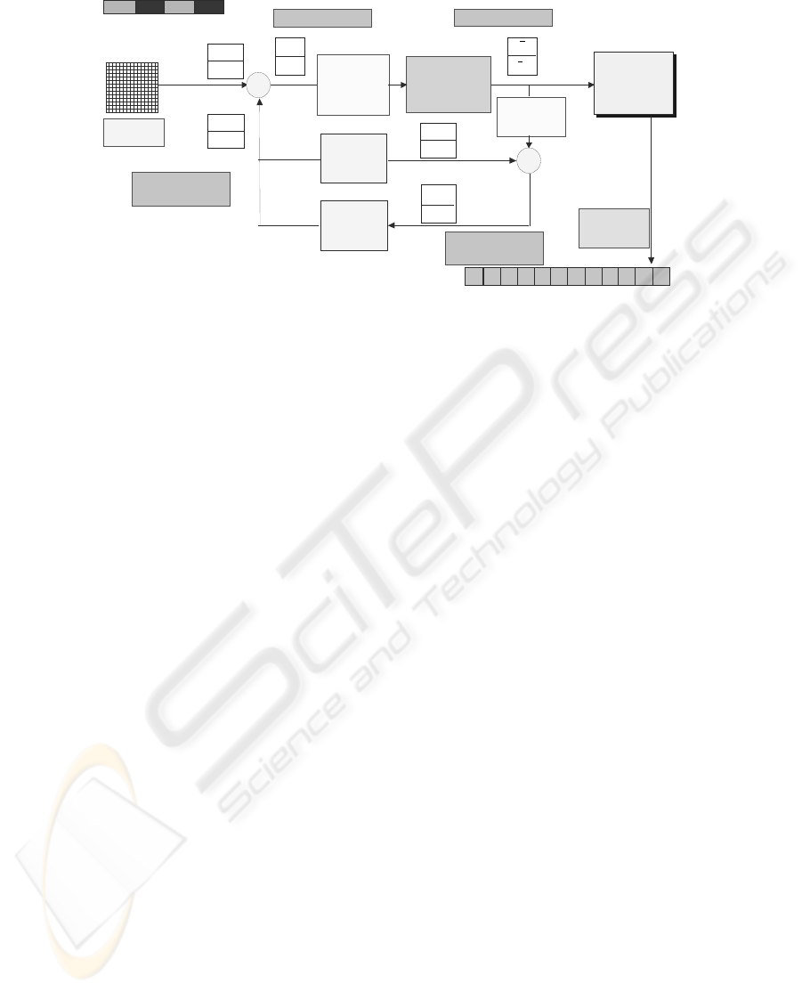
Figure 1: Proposed coding scheme

First, a 2-dimensional Discrete Wavelet Transform

(DWT) is applied and then the DWT coefficients are

quantized. DWT is used because it allows to

describe abrupt changes better than Fourier

transform.

The result is a lossy compression that is perceived as

visually lossless by the Human Visual System

(HVS). Several sub-band coding compression

methods have been introduced by Toi (Toi et alii,

1999) and Le Gall (Le Gall et alii, 1988).

An algorithm (Lee et alii, 2001) for Bayer image

compression based on JPEG (Wallace, 1991) has

been recently proposed. This method, encodes the

image using the JPEG standard. The image is pre-

processed to convert from Bayer to YCbCr format

with 4:2:2 or 4:2:0 sub-sampling. After this

transformation, Y data presents blank pixels, so

JPEG compression cannot be directly applied.

Therefore a simply 45

rotation of Y data is

performed. After the rotation, Y data is localized in

the centre of the image in a rhombus shape by

removing rows and columns containing blank pixel.

The blocks located on the boundaries Y image data

are filled by using a mirroring method before

encoding with JPEG.

All these approaches require appreciable amount of

memory and bandwidth. An efficient compression

technique based on Vector Quantization (VQ)

techniques coupled with consideration on Human

Visual System (HVS) has been proposed recently

(Battiato et alii, 2003). Bayer pattern values are

gathered in groups of two pixels accordingly to their

colour channel and then the generated couple is

quantized with a function considering effects of

“Edge Masking” and “Luma Masking”.

This paper presents an efficient Bayer Pattern lossy

compression technique devised specifically to

reduce the data acquired by the sensor of 40% with a

final low bit rate (about 2:1) and low distortion

(about 50 dB of PSNR).

The paper is organized as follows: Section 2

describes the proposed method. Section 3 presents

the results of the experiments, while conclusions and

final remarks are discussed in Section 4.

2 BAYER PATTERN

COMPRESSION

The proposed algorithm scheme is described in

Figure 1. First, the DPCM algorithm is applied to

compute the difference between the actual and the

predicted pixel values gathered in vectors of two

consecutive elements of the same colour channel.

Prediction is performed assuming the adjacent

samples of the same colour components having

similar brightness values.

The error between the current value and the

prediction is then processed by the “Vector

Mapping” block in order to reduce the symmetry

and lossy compressed through the “Vector

Quantization” block. The vector quantizer has been

designed to discard information not perceivable,

accordingly to psychovisual considerations based on

HVS properties. The quantized values are then taken

as input by the “Code Generation” block that will

yield a 12 bit code. The encoded data is decoded in

order to retrieve the prediction for the next values.

This allows avoiding propagation errors during the

encoding process.

This scheme assumes to process 10-bpp images, so

each couple of 10 bit pixels generates a 12-bit code

with a compression of 12/20 (60%). The same

process can be easily extended to 8 bpp-images.

Bayer

Pattern

Code

Generation

Code

Generation

12 bit code

Vector

Quantization

i+1

−i

Reconstructed

values

1+i

Prediction errors Quantized errors

Predictor

’

i+1

’

i+1

0 11 11 10 00 001 0 11 11 10 00 001

Memory

i-2

’

i-1

’

Predictcted

values

Vector

Mapping

Vector

Inverse

Mapping

ICETE 2004 - WIRELESS COMMUNICATION SYSTEMS AND NETWORKS

326

Next subsections describe with more detail each step

of the co/decoding procedures.

2.1 Step 1: Prediction and

Differential Block

The DPCM step is based on the idea of reducing the

entropy of the source by coding the difference

between the current value and a prediction of the

value itself. In our approach the prediction function

is performed with 2-dimensional vectors obtained

applying VQ. In particular, let (V

, V

) be the vector

to be coded. The second value of the previous vector

i-1

, V

j-1

) is used to build a vector of two identical

components (V

j-1

, V

j-1

) which is the predictor for (V

). This strategy has been chosen because V

j-1

spatially closer to (V

) than V

i-1

and usually closer

samples are statistically more correlated. The error

vectors (e

, e

) are computed as the difference

between the vector to be coded and the prediction

vector:

, e

) =(V

)-(V

j-1

)= (V

-V

j-1

, V

-V

j-1

A typical error distribution for this kind of

prediction scheme is showed in

Figure 1.

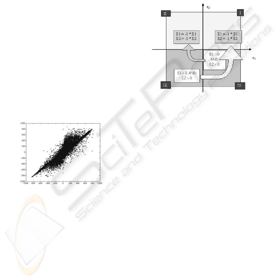
Figure 2: DPCM error spreading.

Observe that a very high percentage of values falls

near the origin, so the used vector quantizer has been

modelled optimizing this distribution.

Note that the prediction function uses, as input, the

restored values that are used as input for the

predictor block in the decompressor. In this way no

errors propagation is present in the compression-

decompression system (

Figure 1 and Figure 7).

2.2 Step 2: Vector Mapping

In the prediction error distribution described above

is evident an odd symmetry. It can be exploited to

reduce the size of the table used for the VQ. In fact

the vectors falling in the third and in the fourth

quadrant can be mapped in the first and in the

second one, so just the two upper quadrants are to be

quantized.

This task is performed by the “Vector Mapping”

block: it checks whether the input vector falls in the

upper part of the diagram or not. In the first case no

changes occur, while, in the other case, the sign of

the values is changed as shown in the Figure 3.

One bit is used in the compressed code in order to

take into account such mapping (see Paragraph 2.4

for details).

Figure 3: Vector Mapping.

2.3 Step 3: Vector Quantization

Given a vector (X

,...,X

) of size N, basic concept of

Vector Quantization (Gray et alii, 1998) can be

described geometrically. The associated binary

representation can be seen as a set of N coordinates

locating a unique point in the N-dimensional space.

The quantization is performed partitioning the space

with N-dimensional cells (e.g. hyperspheres or

hypercubes) with no gaps and no overlaps. As the

point defined by the input vector falls in one of these

cells, the quantization process returns a single vector

associated with the selected cell. Finally, such vector

is mapped to a unique binary representation, which is

the actual output of the vector quantizer. This binary

representation (code) can have fixed or variable

length.

A vector quantizer is said to be “uniform” if the same

quantization step is applied to each vector element,

so that the N-dimensional space is divided into

regular cells. If the space is partitioned into regions

of different size, corresponding to different

quantization step, the quantizer is called “not-

uniform”. The “target” vector is called “codevector”

and the set of all codevectors is the “codebook”. A

grayscale 10 bit image is described by 2-dimensional

vectors of brightness values falling into the range [0,

1023]. In the proposed model, each codevector

BAYER PATTERN COMPRESSION BY PREDICTION ERRORS VECTOR QUANTIZATION

327

represents a 2-dimensional input vector. Moreover,

the proposed algorithm uses a not uniform

quantization according with the properties of HVS.

In particular, two considerations should be taken into

account: the quantization errors are less visible along

the edges and the HVS discriminates better the

details at low luminance levels. Thus, in the areas

near the origin (where the prediction error is low) a

fine quantization is performed and most information

is preserved. On the contrary, in the area far from the

origin, a coarse quantization is applied due to the

presence of boundaries and more information is loss.

Furthermore, since DPCM drifts the values towards

zero, a very high percentile of input samples will fall

in the area around zero.

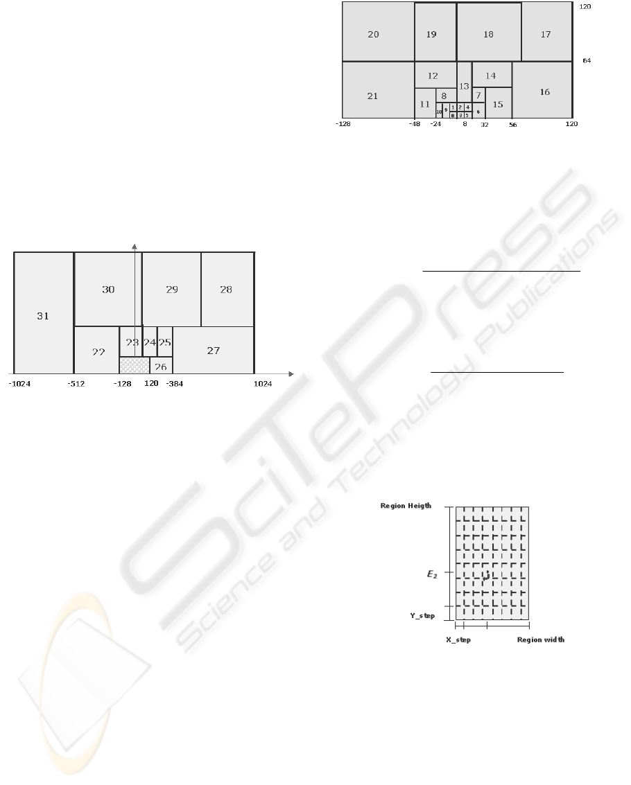
Figure 4: Outer Quantization Regions.

In the testing database used in experiments reported

in this paper containing 130 images, the 65% of

prediction errors are less than 20 and the 80% of

values are less than 38. This information has been

exploited partitioning the two upper quadrants of the

2-dimensional space into regions shaped and

distributed to minimize the quantization error. Each

region has different size and position in the

quantization board and it has been divided into 64

“sub-regions”. Such regions have been obtained

dividing the horizontal and vertical dimension by a

constant number. In this way, bigger regions cover

bigger areas and the quantization is stronger (more

loss of information), while in smaller areas a lighter

quantization is applied and most information is

preserved (Figure 4). The Figure 5 shows an

enlarged image of the quantized region near the

origin.

We assumed that the regions are 32 and that each

region is fragmented into 64 sub-regions (Figure 6).

Figure 5: Inner Quantization Region.

Each vector (e

, e

) to be quantized is

approximated with the nearest couple in the

corresponding sub-region. The quantization step in

the horizontal direction X_step is given by:

onStepQuantizatiHorizontal

gionWidthRe

StepX =_

In the same way, the quantization step in the vertical

direction Y_step is given by:

StepantizationVerticalQu

HeightgionRe

StepY

_ =

Where RegionWidth and RegionHeight are the width

and the height of each region, while

HorizontalQuantizationStep and VerticalQuantiza-

tionStep are the number of partitions in each

direction.

Figure 6: Sub-region partitioning.

The Horizontal and Vertical Quantization Step are set

accordingly to the length of the code and the allowed

distortion in quantization (Figure 6).

2.4 Step 4: Code Generation

The code representing the vector quantized samples

is a fixed length code. It summarizes information

about the vector mapping, the region where the point

falls and the quantization steps applied in each

ICETE 2004 - WIRELESS COMMUNICATION SYSTEMS AND NETWORKS

328

region. The first bit is the “Vector Mapping” bit,

indicating if the swap between upper and bottom

quadrants has happen or not (section 2.2). Next bits

following indicate the index of the region in the

quantization table. The length of this part of the code

depends on the number of regions in the quantization

table. The remaining bits give information on the

number of steps, in both vertical and horizontal

direction inside the region.

In this discussion we assumed that a 12-bits code

should be generated, in order to represent samples

falling in a space partitioned into 32 regions and 64

“sub-regions”. Thus, the code reserves five bits to

index 32 regions and 6 bits to index one of the 64

sub-regions. Different code structure could be

defined if the space partitioning or the target bitrate

change.

2.5 BP Decoding

Decoding procedure consists on three main steps.

The first one is the code evaluation allowing the

extraction of the compressed values. The second one

is the “Inverse Vector Mapping”. It assigns the right

sign to values depending on the inversion flag. Then

the retrieving of the original values is obtained

adding the decoded prediction error to the previously

restored vector. Since the predictor is equal both in

the encoder and the decoder, the predicted values are

equal in the two part of the processes, so there is no

propagation of error during the decoding process.

The decoder block diagram is shown in Figure 7.

Figure 7: Bayer Pattern Decompressor scheme for a pair

of green pels

3 RESULTS

The algorithm has been tested on two sets of images

acquired in different light conditions. A first set,

named “Wide Range Image set”, contains images

acquired by a CMOS-VGA sensor and with a

histogram distributed in almost all the intensity

range for each channel. In the second set the images

have a very narrow histogram. The proposed method

had very good performance with a PSNR of about

56 dB in the first set (Figure 8).

Lower, but still high (about 50 dB) PSNR has been

achieved when the images with a wider range have

been processed (Figure 9). In both cases

compression didn’t introduce perceptible artefacts in

the output images. The algorithm has been compared

with another VQ-based compression method

introduced by S.Battiato et alii in 2003. Both the

approaches yield a fixed-length coding providing a

compression from 10 to 6 bpp.

Figure 8: PSNR comparison between the proposed method

and a classic algorithm on narrow range image set

Figure 9: Figure 10: PSNR comparison between the

proposed method and a classic algorithm on wide range

images.

4 CONCLUSIONS

A new algorithm to compress images acquired by

sensors is presented. The algorithm is oriented to the

compression of the Bayer pattern, the most used

pattern in image acquisition devices.

The technique is based on a predictive schema

where the prediction error is encoded. Each input

Code

evaluation

Code

evaluation

12 bit code

Quantized errors

Reconstructe d

values

0 11 11 10 00 001 0 11 11 10 00 001

1+i

−i

Predictor

’

i+1

’

Memory

Vec tor

Inv erse

Mapping

Vector

Inv erse

Mapping

BAYER PATTERN COMPRESSION BY PREDICTION ERRORS VECTOR QUANTIZATION

329

vector is composed by two adjacent pixels of the

same colour component.

The proposed method allows achieving a

compression of 40% of the input data using a fixed-

length 12-bits code assigned to each couple of 10-

bits input pixel. Moreover, experimental results

showed that compression doesn’t involve a

perceptible loss of quality in the output. As a result,

the bit rate is low and the distortion introduced by

compression is very limited (about 50 dB PSNR).

REFERENCES

R.M. Gray, D.L. Neuhoff, 1998, Quantization, IEEE

Trans. on Information Theory, vol. 44, n. 6.

R.C. Gonzales, R.E. Woods, 1993, Digital Image

Processing, Addison Wesley, pp.358-374.

B.E. Bayer, 1976, Color Imaging Array, U.S. Patent

3,971,065.

Hynix CMOS Image Sensor Application Note 2002,

Endpoints SE401 Demokit Information,

http://www.hynix.com/datasheet/pdf/system_ic/sp/SE

401_Demokit.pdf

T. Acharya, L.J. Karam, F. Marino, 2000 Compression of

Color Images Based on a 2-Dimensional Discrete

Wavelet Transform Yielding a Perceptually Lossless

Image, U.S.Patent 6,154,493.

T.Toi, M.Ohita, 1999, A Subband Coding Technique for

Image Compression in Single CCD Cameras with

Bayer Color Filter Arrays, IEEE Transaction on

Consumer Electronics, Vol.45, N.1, pp.176-180.

Sang-Yong Lee, A. Ortega, 2001, A Novel Approach of

Image Compression in Digital Cameras With a Bayer

Color Filter Array, In Proceedings of ICIP 2001 –

International Conference on Image Processing – Vol.

III 482-485 - Thessaloniki, Greece.

G. K. Wallace, 1991, The JPEG still picture compression

standard, Communications of the ACM 34(4), pp.

30-44.

Le Gall, A. Tabatabai, 1988, Subband Coding of Digital

ImagesUsing Symmetric Shor Kernel Filters and

Arithmetic Coding Techniques, in Proceedings of the

ICASSP 88 Conference, (New York), pp. 761-764.

S. Battiato, A. Buemi, L. Della Torre, A. Vitali, 2003,

“Fast Vector Quantization Engine for CFA Data

Compression”, In Proceedings of IEEE-EURASIP

Workshop on Nonlinear Signal and Image Processing,

NSIP, Grado, Italy.

ICETE 2004 - WIRELESS COMMUNICATION SYSTEMS AND NETWORKS

330