
DATABASES REDUCTION
Roberto Ruiz and Jos
´
e C. Riquelme and Jes
´
us S. Aguilar-Ruiz
Department of Computer Science. University of Seville
Avda. Reina Mercedes s/n. 41012-Sevilla. Spain.
Keywords:
Data mining, preprocessing technics, database reduction, feature selection, data set editing.
Abstract:
Progress in digital data acquisition and storage technology has resulted in the growth of huge databases. Nev-
ertheless, these techniques often have high computational cost. Then, it is advisable to apply a preprocessing
phase to reduce the time complexity. These preprocessing techniques are fundamentally oriented to either of
the next goals: horizontal reduction of the databases or feature selection; and vertical reduction or editing. In
this paper we present a new proposal to reduce databases applying sequentially vertical and horizontal reduc-
tion technics. They are based in our original works, and they use a projection concept as a method to choose
examples and representative features. Results are very satisfactory, because the reduced database offers the
same intrinsic performance for the later application of classification techniques with low computational re-
sources.
1 INTRODUCTION
The data mining researchers, especially those dedi-
cated to the study of algorithms that produce knowl-
edge in some of the usual representations (decision
lists, decision trees, association rules, etc.), usually
make their tests on standard and accessible databases
(most of them with small size). The purpose is to
independently verify and validate the results of their
algorithms. Nevertheless, these algorithms are mod-
ified to solve specific problems, for example real
databases that contain much more information (tens
of attributes and tens of thousands of examples) than
standard ones used in training. Therefore, applying
these data mining techniques is a task that takes a lot
of time and memory size, even with the capability of
current computers, which make the adaption of the al-
gorithm to solve the problem extremely difficult.
Therefore, it is important to apply preprocessing
techniques to the databases. These preprocessing
techniques are fundamentally oriented to one of the
next goals: feature selection methods (eliminating
non-relevant attributes) and editing algorithms (re-
duction of the number of examples). Existing meth-
ods solve one out of the two aforementioned prob-
lems.
In this paper we present a new approach to reduce
databases in both directions. This is due to sequential
application of vertical and horizontal reduction tech-
niques. They both are based in our original works,
and they use a projection concept as a method to
choose examples and representative features.
2 VERTICAL REDUCTION
2.1 Related work
Editing methods are related to the nearest neigh-
bours (NN) techniques (Cover and Hart, 1967). Some
of them are briefly cited in the following lines.
Hart (Hart, 1968) proposed to include in the subset
S, those examples of the training set T whose classi-
fication with respect to S are wrong using the near-
est neighbour technique, so that every member of T
is closer to a member of S of the same class than to
a member of S of a different class; Aha et al. pro-
posed a variant of Harts method; Wilson (Wilson,
1972) proposed to eliminate the examples with in-
correct K-NN classification, so that each member of
T is removed if it is incorrectly classified with the
N nearest neighbours; (Tomek, 1976) extended the
idea of Wilson eliminating the examples with incor-
rect classification from any i=1 to N, where N is the
maximum number of neighbours to be analysed; the
work of (Ritter et al., 1975) extended Harts method
and every member of T must be closer to a mem-
ber of S of the same class than to any member of T.
Other variants are based on Voronoi diagrams (Klee,
98
Ruiz R., C. Riquelme J. and S. Aguilar-Ruiz J. (2004).
DATABASES REDUCTION.
In Proceedings of the Sixth International Conference on Enterprise Information Systems, pages 98-103
DOI: 10.5220/0002632300980103
Copyright
c
SciTePress
1980), Gabriel neighbours (two examples are said to
be Gabriel neighbours if their diametrical sphere does
not contain any other examples) or relative neigh-
bours (Toussaint, 1980) (two examples p and q are rel-
ative neighbours if for all other examples x in the set,
is true the expression dist(p,q)¡maxdist(p,x),dist(q,x).
All of these techniques need to calculate distances be-
tween examples, which is rather time consuming. If
N examples with M attributes are considered, the first
methods take O(MN
2
) time, the Ritters algorithm is
O(MN
2
+N
3
); the Voronoi neighbours, Gabriel neigh-
bours and relative neighbours are O(MN
3
).
The most important characteristics of our editing
algorithm, called EOP (Aguilar et al., 2000) (Editing
by Ordered Projection), are:
• Considerable reduction of the number of examples.
• Lower computational cost O(MNlog N) than other
algorithms.
• Absence of distance calculations.
• Conservation of the decision boundaries, especially
interesting for applying classifiers based on axis-
parallel decision rules (like C4.5).
2.2 Editing
If we choose a region where all examples inside have
the same class, perhaps we could select some of
them, which are not decisive, in order to establish the
boundaries of the region. For example, in two dimen-
sions we need a maximum of four examples to de-
termine the boundaries of one region. In general, in
d-dimensions we will need 2d examples, maximum.
Therefore, if a region has more than 2d examples, we
could reduce the number of them.
This is the main idea of our algorithm: to elimi-
nate the examples that are not in the boundaries of the
regions to which they belong. The aim is to calcu-
late which set of examples could be covered by a pure
region and then eliminate those inside that are not es-
tablishing the boundaries. A region is pure if all the
examples inside have the same class.
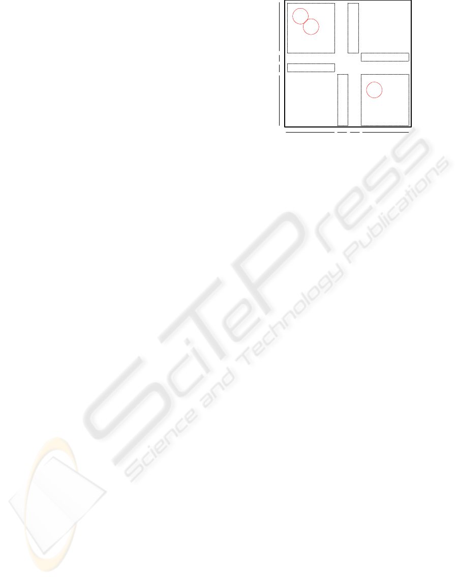
Consider the situation depicted in Figure 1: the pro-
jection of the examples on the abscissa axis produces
four ordered sequences {I; P; I; P} corresponding to
the examples {[9; 3; 5; 1; 11]; [8]; [7]; [4; 6; 2; 12;
10]}. Identically, with the projection on the ordinate
axis, we can obtain the sequences {P; I; P; I} formed
by the examples {[12; 10; 8; 6; 4]; [11]; [2]; [9; 7;
5; 3; 1]}. Each sequence represents a rectangular re-
gion as a possible solution of a classier (a rule) and
the initial and final examples of the sequence (if it
has only one, it is simultaneously the initial and the
final one) represent the lower and upper values for
each coordinate of this rectangle. For example, there
is a rectangle formed by the examples {1; 3; 5; 7; 9}.
4
1
3
9
7
11
8
2
6
5
10
12
I
P
P
I
I P I P
Figure 1: Results of applying EOP
This region needs the examples {9; 7} to establish the
boundaries of a dimension and the examples {1; 9}
for another one. Therefore, the remaining examples
will be candidates to be eliminated because they are
never boundaries. The idea is best understood by an-
alyzing the non-empty regions obtained by means of
projections on every axis and deleting the examples
that are not relevant so as to establish the boundaries
of a rule.
In regards to the analysis of this editing method,
we have dealt with eighteen databases from the UCI
repository (Blake and Merz, 1998). To show the per-
formance of our method we have used C4.5 (Quinlan,
1993) and k–NN (Hart, 1968) before and after apply-
ing EOP. The obtained results (Riquelme et al., 2003)
prove the validity of the method.
Table 1: EOP algorithm
Input: E training (N ex., M att.)
Output: E reduced (L ex., M att.)
for each example e ∈ E
weakness(e) = 0
for each attribute a
sort E in increasing order
for each example e ∈ E
if it is NOT border
increase weakness(e)
for each example e ∈ E
if weakness = M
delete register e
3 HORIZONTAL REDUCTION
3.1 Related work
Depending on the evaluation strategies, feature selec-
tion algorithms can generally be placed into one of
DATABASES REDUCTION
99

two broad categories: wrappers, Kohavi (Kohavi and
John, 1997), which employ a statistical re-sampling
technique (such as cross validation) using the actual
target learning algorithm to estimate the accuracy of
feature subsets. This approach has proved to be use-
ful but is very slow to execute because the learning
algorithm is called upon repeatedly. Another option
called filter, operates independently of any learning
algorithm. Undesirable features are filtered out of the
data before induction begins. Filters use heuristics
based on general characteristics of the data to eval-
uate the merit of feature subsets. As a consequence,
filter methods are generally much faster than wrapper
methods, and, as such, are more practical for use on
data of high dimensionality. LVF (Liu and Setiono,
1996) use class consistency as an evaluation measure.
One method called Chi2 (Liu and Setiono, 1995) real-
ize selection by discretization . Relief (Kira and Ren-
dell, 1992) works by randomly sampling an instance
from the data, and then locating its nearest neighbour
from the same and opposite class. Relief was origi-
nally defined for two-class problems and was later ex-
panded as ReliefF (Kononenko, 1994) to handle noise
and multi-class data sets, and RReliefF handles re-
gression problems. Other authors suggest Neuronal
Networks for attribute selector. In addition, learn-
ing procedures can be used to select attributes, like
ID3 (Quinlan, 1986), FRINGE (Pagallo and Haussler,
1990) and C4.5 (Quinlan, 1993) as well as methods
based on correlations like CFS (Hall, 1997).
The most important characteristics of our feature
selection algorithm, called SOAP (Ruiz et al., 2002)
(Selection of Attributes by Projection), are very simi-
lar to that of EOP.
3.2 Feature selection
In this paper, we propose a new feature selection cri-
terion not based on measures calculated between at-
tributes, or complex and costly distance calculations.
This criterion is based on a unique value called NLC.
It relates each attribute with the label used for classifi-
cation. This value is calculated by projecting data set
elements onto the respective axis of the attribute (or-
dering the examples by this attribute), then crossing
the axis from the beginning to the greatest attribute
value, and counting the Number of Label Changes
(NLC) produced.
Consider the situation depicted in Figure 2: the pro-
jection of the examples on the abscissa axis produces
three ordered sequences {O; E; O} corresponding to
the examples {[1,3,5],[8,4,10,2,6],[7,9]}. Identically,
with the projection on the ordinate axis, we can ob-
tain the sequences {O; E; O; E; O; E} formed by the
examples {[8],[7,5],[10,6],[9,3],[4,2],[1]}. Then, we
calculate the Number of Label Changes, NLC. Two
for the first attribute and five for the second.
E 8
7
5
10
6
9
3
4
2
O 1
O E O
O
E
O
E
Figure 2: Results of applying SOAP
We conclude that it will be easier to classify by at-
tributes with the smallest number of label changes. If
the attributes are in ascending order according to the
NLC, we obtain a ranking list with the better attributes
from the point of view of the classification.
We have dealt with eighteen databases from the
UCI repository [3]. To show the performance of our
method we have used k-NN and C4.5 before and af-
ter applying EOP. Results obtained (Ruiz et al., 2002)
prove the validity of the method.
Table 2: SOAP algorithm
Input: E training (N ex., M att.)
Output: E reduced (N ex., K att.)
for each attribute a
sort E in increasing order
count label changes
ranking attributes by NLC
choose the k first attributes
4 INTEGRATION OF
REDUCTION TECHNIQUES
The size of a data set can be measured in two dimen-
sions, number of features and number of instances.
Both can be very large. This enormity may cause se-
rious problems to many data mining systems.
Our approach is to reduce the database in the two
directions, vertically and horizontally, applying the
aforementioned algorithms sequentially.
The algorithm is very simple and efficient. The
computational cost of EOP and SOAP is O(m × n
× log n), being the lowest of its category. Therefore,
the new algorithm is efficient too.
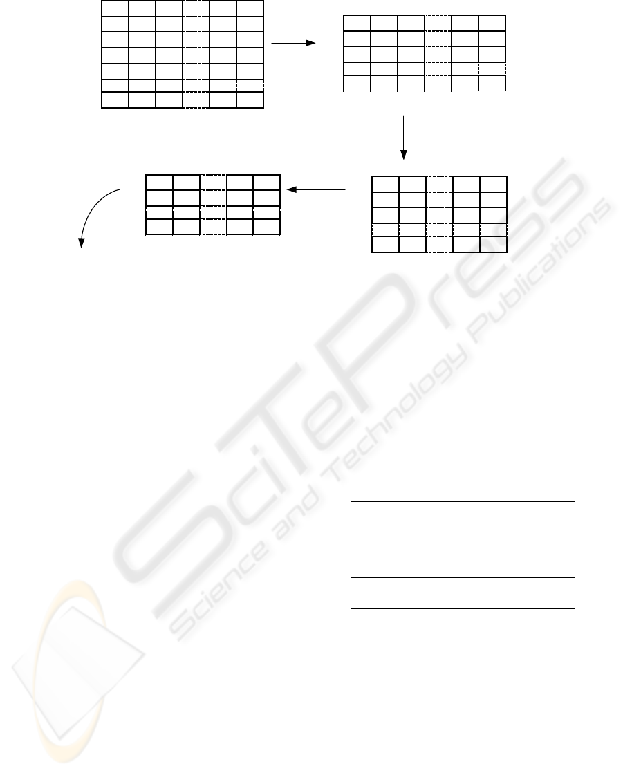
Figure 3 shows the process to reduce a database
with two thousand examples and forty one attributes,
the last feature being the class. There are three posi-
ble labels A,B,C. At the beginning, vertical reduction
is applied with the algorithm EOP. The number of ex-
amples decreases to three hundred and fifty. Then,
ICEIS 2004 - ARTIFICIAL INTELLIGENCE AND DECISION SUPPORT SYSTEMS
100
EPO
Horizontal
reduction
SOAP
Vertical
reduction
EPO
Vertical
reduction
SOAP
A
1
A
2
A
3
...
A
40
Class
R
1
44 Hi 5.96 54 A
R
2
7 Hi 6.88 24 A
R
3
23 No 4.20 18 B
R
4
52 Lo 9.53 30 C
R
5
85 No 7.33 22 A
...
R
2000
59 Lo 3.21 81 B
BD: 2000 ex. x (40 att. + class)
A
1
A
2
A
3
...
A
40
Class
R
1
44 Hi 5.96 54 A
R
4
52 Lo 9.53 30 C
R
5
85 No 7.33 22 A
...
R
458
37 No 8,36 34 B
BD: 350 ex. x 41 att.
A
1
A
3
...
A
15
Class
R
1
44 5.96 V A
R
4
52 9.53 F C
R
5
85 7.33 V A
...
R
458
37 8,36 V B
BD: 350 ex. x 9 att.
A
1
A
3
...
A
15
Class
R
1
44 5.96 V A
R
5
85 7.33 V A
...
R
385
65 6.48 F C
BD: 334 ex. x 9 att.
Figure 3: Database reduction process
Table 3: Main algorithm
Input: E training (N ex., M att.)
Output: E reduced (L ex., K att.)
E’ = EPO(E)
while ( E’ <> E )
E = SOAP(E’)
E’ = EPO(E)
endwhile
E’ = SOAP(E)
the most relevant attributes are chosen by mean of the
SOAP algorithm. The number of features decreases
to nine attributes. The one and the other algorithm are
applied using EOP as a stopping criterion, until a new
execution does not reduce the data set.
5 EXPERIMENTS
In this section, we want to analyze our algorithm with
a large data set. We would like obtain a set with a
considerable size (more than twenty thousand exam-
ples), and with low missing values, and where we do
not know the attributes’ relevancy. This is not easy to
find and we decided to create one. We considered a
large enough database would be with forty thousand
examples and forty features, and it would present an
adequate difficulty to prove our algorithm in the de-
sired environment.
We generate examples randomly, and we label
them according to the same given rules. At the end,
we add a percentage of examples with noise. We try to
set the minimum number of parameters (Table 5), and
the other parameters are solved randomly. Therefore,
there are three important fixed parameters: Number of
rules (thirty-five); Conditions used in each rule (four);
And the set of possible labels (five). We label exam-
ples consecutively (rule 0: label A, rule 1: label B,...,
rule 5: label A,...). Then, each label can be obtained
for seven different rules (35 rules / 5 classes = seven).
Table 4: Parameters
Examples 40000
Attributes 40
Rules 35
Conditions x rule 4
Labels 5
35 rules x 4 = 140 conditions
35 rules / 5 labels = 7
There are four attributes in each rule (one for each
condition Table 5) and they are constants. But inter-
vals of each attribute are obtained randomly within
some fixed limits. One rule is different than the rest
at least in two attributes, then, we offer a wide range
of regions.
Condition : (li < att < hi)
att : constant
li, hi : random
∀X, Y #(ruleX ∩ ruleY ) 6 2atts.
Consider that one attribute is more relevant than
another if we use it more times in the set of rules,
DATABASES REDUCTION
101
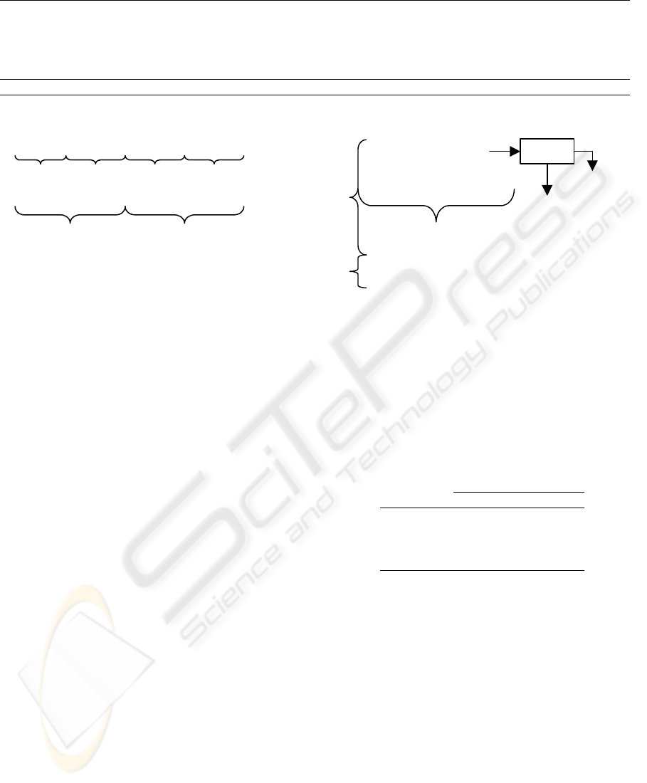
Table 5: Rules
rule 1 condition1 AND condition2 AND condition3 AND condition4 THEN label A
rule 2 condition5 AND condition6 AND condition7 AND condition8 THEN label B
rule 3 condition9 AND condition10 AND condition11 AND condition12 THEN label C
. . . . . . AND . . . AND . . . AND . . . THEN . . .
rule 35 condition137 AND condition138 AND condition139 AND condition140 THEN label E
Ex. [lo1<att1<hi1] AND [lo2<att2<hi2] AND [lo6<att6<hi6] AND [lo9<att9<hi9] THEN label A
A
1
,... A
5
,A
6
,...,A
10
,A
11
,...,A
15
,A
16
,...,A
20
14 veces
x 5 atts
= 70
8 veces
x 5 atts
= 40
4 veces
x 5 atts
= 20
2 veces
x 5 atts
= 10
relevants less relevants
redundants
Irrelevants
+
Figure 4: Relevance of the attributes
and we want to obtain four groups of well sepa-
rated attributes. They are relevant, less relevant, re-
dundant and dummy attributes with ten attributes in
each group. The first and the second group (rele-
vant and less relevant) are divided into two subgroups,
with five attributes more relevant than the other five.
Therefore, we have six different groups of attributes.
The importance of the attributes is related to the
number of times that it appears in the set of rules.
Rules are built by four of the twenty attributes, those
who belong to the relevant and less relevant group.
All in all, the distribution of the attributes in the set
of rules is as follows: fourteen times five attributes
belonging to the relevant group, and eight times the
other attributes of the group. Four times five attributes
belonging to the less relevant group, and two times the
other attributes of this group.
The first step (Figure 5) in the process followed to
generate the database is to obtain the value of twenty
from forty attributes randomly (belonging to relevant
and less relevant group). Then, we filter them through
the set of rules and it is classified with a label. If an
example validate more than one rule with a different
label, then it is thrown out. In the contrary case, we set
the value of the rest of the attributes; ten features ob-
tained randomly, the irrelevant attributes, and another
ten according to some part of the other thirty attributes
(redundant group). This process is repeated until the
database is full. At the end of the process, we add a
number of register with noise (10%), i.e. the value of
each attribute is obtained randomly (label included).
The only thing remaining is to mix the attributes of
the different groups.
We conclude that to obtain a learning model from
the data set generated is very complex, i.e. if we try
Random(A
1
A
2
,...,A
20
)
36000 ex.
Random(A
1
A
2
,A
3
,...,A
40
,class)
4000 ex.
rules
Class
Throw out
f(A
1
A
2
,A
3
,...,A
30
)= (A
31
A
32
,A
33
,...,A
40
)
Random(A
21
A
22
,A
23
,...,A
30
)
1label
>1
Figure 5: Process to generate de database
to generate a set of decision rules or decision tree
from the database, the model of accuracy rate from
the training set will be low. Therefore, preprocessing
techniques must be very robust and efficient, because
of the size of the data.
Table 6: Results obtained
Original Reduced
Examples 40000 22451
Attributes 40 5
C4.5 % 53.33 58.45
C4.5 size 9897 8011
Table 5 shows, after the generation of the data
set with 40000 examples and 40 attributes, we ap-
ply the classifier C4.5. and we obtain a tree with a
size 9897, and 21334 well classified examples, this
is 53.33% of the data. Now we apply our new algo-
rithm, and we obtain a reduced data set with 22451
examples and 5 attributes. We reduce the number
of examples to 56% of the original examples and
13% of the original attributes. In general, the size
of the database (40000x40=1600000) is reduced to
(22451x5=112255). Our method reduces the data by
93% of the original size, leaving us with 7% of the
original data ().
Applying C4.5 to the reduced database, i.e. we
use 7% of the original data. We obtain a smaller tree
size, 8011 nodes. If we classify the 40000 examples,
the accuracy is 58.45%, better than with the origi-
ICEIS 2004 - ARTIFICIAL INTELLIGENCE AND DECISION SUPPORT SYSTEMS
102

nal data. Therefore, this new method is robust. We
conclude that a classifier like C4.5 generates a bet-
ter result when an effective preprocessing technique
is used.
6 CONCLUSIONS
In this paper we present an integration technique of
database reduction algorithms. This integration is
based on two techniques applied sequentially. The
first is a reduction of examples method (editing or
vertical reduction), and the second one is a reduction
of attributes algorithm (feature selection or horizontal
reduction). Both techniques are valid in previous pa-
pers, and they are efficient techniques, because their
computational costs are the lowest of its respective
categories.
Given the satisfactory results, using a specifically
generated database with extreme complexity, we can
state that the of integration approach of the two re-
duction techniques (horizontal and vertical) is very
interesting from the data mining techniques applica-
tion point of view.
Results show a very important data reduction, 93%.
Nevertheless, the quality of the information is the
same with only 7% of the original data. A model is
generated based on a decision tree, and its accuracy is
slightly better than the accuracy obtained with all the
data.
Our work is going to be oriented to the integration
of other reduction techniques and the application to
real world data sets.
ACKNOWLEDGEMENTS
This work has been supported by the Spanish Re-
search Agency CICYT under grant TIC2001-1143-
C03-02.
REFERENCES
Aguilar, J. S., Riquelme, J. C., and Toro, M. (2000). Data set
editing by ordered projection. In Proceedings of the
14
th
European Conference on Artificial Intelligence,
pages 251–255, Berlin, Germany.
Blake, C. and Merz, E. K. (1998). Uci repository of ma-
chine learning databases.
Cover, T. M. and Hart, P. E. (1967). Nearest neighbor pat-
tern classification. IEEE Transactions on Information
Theory, IT-13(1):21–27.
Hall, M. (1997). Correlation-based feature selection for
machine learning. PhD thesis, University of Waikato,
Hamilton, New Zealand, Department of Computer
Science.
Hart, P. (1968). The condensed nearest neighbor rule. IEEE
Transactions on Information Theory, 14(3):515–516.
Kira, K. and Rendell, L. (1992). A practical approach to
feature selection. In International Conference on Ma-
chine Learning, pages 368–377.
Klee, V. (1980). On the complexity of d-dimensional
voronoi diagrams. Arch. Math., 34:75–80.
Kohavi, R. and John, G. H. (1997). Wrappers for feature
subset selection. Artificial Intalligence, 1-2:273–324.
Kononenko, I. (1994). Estimating attributes: Analysis and
estensions of relief. In European Conference on Ma-
chine Learning, pages 171–182.
Liu, H. and Setiono, R. (1995). Chi2: Feature selection and
discretization of numeric attributes. In Proceedings of
the Seventh IEEE International Conference on Tools
with Artificial Intelligence.
Liu, H. and Setiono, R. (1996). Feature selection and clas-
sification: a probabilistic wrapper approach. In Pro-
ceedings of the IEA-AIE.
Pagallo, G. and Haussler, D. (1990). Boolean feature
discovery in empirical learning. Machine Learning,
5:71–99.
Quinlan, J. (1986). Induction of decision trees. Machine
Learning, 1:81–106.
Quinlan, J. R. (1993). C4.5: Programs for machine learn-
ing. Morgan Kaufmann, San Mateo, California.
Riquelme, J., Aguilar-Ruiz, J. S., and Toro, M. (2003).
Finding representative patterns with ordered projec-
tions. Pattern Recognition, 36(4):1009–1018.
Ritter, G., Woodruff, H., Lowry, S., and Isenhour, T. (1975).
An algorithm for a selective nearest neighbor deci-
sion rule. IEEE Transactions on Information Theory,
21(6):665–669.
Ruiz, R., Riquelme, J., and Aguilar-Ruiz, J. S. (2002).
Projection-based measure for efficient feature selec-
tion. Journal of Intelligent and Fuzzy System, 12(3-
4):175–183.
Tomek, I. (1976). An experiment with the edited nearest-
neighbor rule. IEEE Transactions on Systems, Man
and Cybernetics, 6(6):448–452.
Toussaint, G. T. (1980). The relative neighborhood graph
of a finite planar set. Pattern Recognition, 12(4):261–
268.
Wilson, D. (1972). Asymtotic properties of nearest neigh-
bor rules using edited data. IEEE Transactions on Sys-
tems, Man and Cybernetics, 2(3):408–421.
DATABASES REDUCTION
103
