TERRAIN CLASSIFICATION FOR OUTDOOR AUTONOMOUS

ROBOTS USING SINGLE 2D LASER SCANS

Robot perception for dirt road navigation

Morten Rufus Blas, Søren Riisgaard, Ole Ravn, Nils A. Andersen, Mogens Blanke, Jens C. Andersen

Section of Automation, Ørsted

•

DTU, Technical University of Denmark, DK 2800 Kgs. Lyngby,Denmark

Keywords: terrain classification, obstacle detection, road following, laser scanner, classifier fusion.

Abstract: Interpreting laser data to allow autonomous robot navigation on paved as well as dirt roads using a fixed

angle 2D laser scanner is a daunting task. This paper introduces an algorithm for terrain classification that

fuses four distinctly different classifiers: raw height, step size, slope, and roughness. Input is a single 2D

laser scan and output is a classification of each laser scan range reading. The range readings are classified

as either returning from an obstacle (not traversable) or from traversable ground. Experimental results are

shown and discussed from the implementation done with a department developed Medium Mobile Robot

and tests conducted in a national park environment.

1 INTRODUCTION

Safe autonomous navigation in unstructured or semi-

structured outdoor environments presents a

considerable challenge. Solving this challenge

would allow applications within many areas such as

ground-based surveillance, agriculture, as well as

mining.

To achieve this level of autonomy, a robot must

be able to perceive and interpret the environment in

a meaningful way. Limitations in current sensing

technology, difficulties in modelling the interaction

between robot and terrain, and a dynamically

changing unknown environment all makes this

difficult.

Imperative for successful and safe autonomous

navigation is the identification of obstacles which

either can be damaged or hurt, or in turn can disable

or cause damage to the robot. Analogous to this it

must also be possible to identify traversable terrain

(e.g. the road). Bertozzi and Broggi (1997) argues

that this problem can be divided into lane following

and obstacle detection. This paper concentrates on

the detection of obstacles.

Much current work in laser scanner classification

tends to focus on using 3D laser scanners, vision or a

combination of 3D laser scanners and vision.

Vandapel (2004) used a 3D laser scanner to classify

point clouds into linear features, surfaces, and

scatter. Classification was based on a learnt training

set. Montemerlo and Thrun (2004) identified

navigable terrain using a 3D laser scanner by

checking if all measurements in the vicinity of a

range reading had less than a few centimetres

deviation. Wallace et al (1986) used a vision-based

edge detection algorithm to identify road borders.

Jochem et. Al (1993) followed roads using vision

and neural networks. Macedo et al (2000) developed

an algorithm that distinguished compressible grass

(which is traversable) from obstacles such as rocks

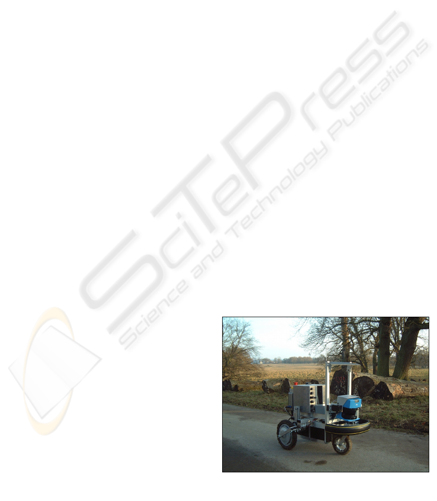
Figure 1: The robot platform tested in the dirt-road semi-

structured environment from a Danish national park

347

Rufus Blas M., Riisgaard S., Ravn O., A. Andersen N., Blanke M. and C. Andersen J. (2005).

TERRAIN CLASSIFICATION FOR OUTDOOR AUTONOMOUS ROBOTS USING SINGLE 2D LASER SCANS - Robot perception for dirt road

navigation.

In Proceedings of the Second International Conference on Informatics in Control, Automation and Robotics - Robotics and Automation, pages 347-352

DOI: 10.5220/0001176003470352

 SciTePress

using spatial coherence techniques with an omni-

directional single line laser.

Wettergreen et al (2005) extracted three metrics

from stereovision data and used these to traverse a

rock field. Iagnemma et al (2004) followed quite

another route and proposed a tactile and vibration-

based approach to terrain classification.

This paper proposes a terrain classification

algorithm that discriminates between obstacles and

traversable terrain using a fixed 2D laser scanner as

the main sensor. This is notoriously harder than

using 3D sensor inputs as there is much less

information available.

In the classification algorithm proposed here, four

essential environment features are associated with

signatures in the 2D laser scan range readings, and

classification is done using a combined classifier on

the extracted features. The salient features looked at

are: terrain height, terrain slope, increments in

terrain height, and variance in height across the

terrain.

This work is a contribution towards demonstrating

that it will become feasible to achieve autonomy

over long distances (>4km) in a natural outdoor

terrain using only a 2D laser scanner for terrain

classification.

The paper shows results of testing the classifier

on the Medium Mobile Robot (MMR) platform from

the Technical University of Denmark on various

paved and dirt roads in a national park (see Figure

1). The quality of classification is discussed for

different cases of natural environment encountered

in the tests. The contribution of the paper is to

demonstrate that the proposed classification

techniques suffice to navigate the MMR safely and

to demonstrate that the proposed method is robust to

the variation encountered in the natural environment

using simple equipment: 2D laser scanner, a cheap

commercial GPS sensor and odometry.

2 TERRAIN CLASSIFICATION

The terrain classification algorithm combines four

distinctly different terrain classifiers: raw height,

step size, slope, and roughness.

Input for each run of the algorithm is a single

laser scan. Output as stated in the Introduction is a

classification for each range reading as returning

from either an obstacle or as traversable terrain. The

terrain classifiers all work on point statistics.

2.1 Coordinate System

On the MMR the laser scanner is tilted at 8° down

towards the ground and gives 180 range readings in

a 180° frontal arc. Only the range readings in a 120°

arc in front of the robot were used for terrain

classification as this approximately corresponds to

which range readings would hit the ground with the

given scanner tilt.

Each laser scan range reading is converted to a

3D point expressed in the vehicle frame. The

vehicle stands in (0, 0, 0). Assuming the robot is

standing on level ground then up (height) is the Z-

axis in the positive direction. The robot looks out

the positive Y-axis, and the X-axis increases towards

the right of the robot. The raw height and step size

classifier only look at the height (Z-axis).

In the following sections P will denote a set of

range readings converted to 3D points. The

hypothesis is that each 3D point can be mapped to

either belonging to an obstacle or traversable terrain.

This is explained in Eq. (1).

()

()\()

Hobstacle P

traversable P H obstacle

⊆

(1)

A single element of

P is denoted

p where i

represents the range reading angle (inside the 180°

frontal arc). The coordinates of a point are given by

(, , )

iiyiz

pppp

. The conversion from range

readings to 3D coordinates is shown in Eq. (2).

range is the measured range at angle i .

tilt

is the

angle the laser scanner is tilted (in our case 8°).

height

S is the height the laser scanner is mounted at

relative to the plane of the robots wheel-base (on the

MMR this is 0.41m).

*cos( )

cos( )* *sin( )

sin( ) * *sin( )

height

px range i

py range i

i tilt i

pz range i S

itilt i

(2)

2.2 Raw Height

This classifier looks at the height of each range

reading (point) in the vehicle frame. If a point is

higher or lower (on the Z-axis) than a value decided

by a height threshold then the point is labelled as

returning from an obstacle. In the tested system if a

point had a height of ±20cm it was labelled as an

ICINCO 2005 - ROBOTICS AND AUTOMATION

348

obstacle. In practice its purpose is to identify

obstacles such as people, tree trunks and pits.

Obstacles inside the ±20cm thresholds cannot be

detected. The robot has no sensors to measure pitch

and yaw of the laser scanner relative to the ground

surface. As such, the height thresholds are chosen to

allow for variations in measured height of the

ground due to lack of attitude determination. The

classifier is shown in Eq. (3) where height

max

and

height

min

are the height thresholds.

max

()

min

pheight

Hobstacle p P

pheight

⎧⎫

⎪⎪

=∈

⎨⎬

∨<

⎪⎪

⎩⎭

(3)

Here, the threshold

min

0height < enables

detection of non-traversable cavities in the ground.

2.3 Step Size

A step size classifier looks at the difference in height

between neighbouring points where neighbouring is

defined as a range within 1° of the specific point. If

the difference in height is higher than a threshold

(here 5 cm) a terrain step is detected that is too high

for the robot to traverse. The algorithm labels both

points that form the border between the step as

obstacles. As it only looks at the step size,

neighbouring points from an obstacle with similar

height may be erroneously labelled as traversable.

The 5 cm threshold was set based on the robot’s

physical specifications, the limiting factor being that

the front wheel cannot reliably climb anything taller.

The classifier is shown in Eq. (4) where step

max

represents the threshold for difference in height.

()

max

(1)

max

(1)

H obstacle

pp step

⎧⎫

−>

⎪⎪

−

⎪⎪

∈

⎨⎬

⎪⎪

∨− >

⎪⎪

⎩⎭

(4)

2.4 Slope

Slope classification aims at identifying terrain which

has too high an incline to be traversed. The

classification is done by calculating a 2D line fit

using least squares around a point sample. For each

point, the neighbouring points within ±2° are used.

The least squares line is then calculated using the X

and Z-axis values. The point examined is

subsequently classified based on its slope. If

exceeding a limit slope

max

= ±0.1 it is classified as

belonging to terrain that is too steep for the robot

and is labelled as an obstacle. The assumption here

is that the best-fit line approximates the steepness of

the terrain around this point sample. The value of

±0.1 was chosen for two reasons. First, it represents

what the robot can physically handle. Secondly, it

keeps the robot on reasonably level ground where

lack of attitude determination is less critical. The

classifier can be seen in Eq. (5) where slope

max

is the

slope threshold.

[]

{}

(2) (2)

and

a singular value decomposition

; ;

, ,... last column of ;

;

()

max

ix iz

TT T

iven

AUDV UU VV I

cc c V

let

calculate

H obstacle p P a slope

−−

⎡⎤

⎢⎥

⎣⎦

===

=−

=∈ >

###

(5)

2.5 Roughness

The roughness classifier looks at the variance in

height in the vicinity of a specific point. The

purpose is to identify areas with low variance as

these areas are more likely to be easily traversable.

For example, heavy underbrush in a forest may have

a high variance; a flat road will appear as a region of

points with a low variance. Trend removal is also

essential as a slightly sloping surface relative to the

vehicle frame may give a high variance in height

relative to the zero height plane {Z|Z=0}. The

variance in height is hence calculated relative to a

2D best-fit line. This line is calculated in the same

manner as in the slope classifier. The variance is

then calculated as the shortest distance from each

point (using again the two neighbouring points on

either side of the point) to the best-fit line using only

the X and Z-axis coordinates. If the variance in a

point sample in this method was found to be larger

than variance

max

= 2.5e-10 the point was labelled as

an obstacle. This classifier can give more accurate

results than the other classifiers (see Table 1) but it

cannot stand alone since, for example, a flat wall

TERRAIN CLASSIFICATION FOR OUTDOOR AUTONOMOUS ROBOTS USING SINGLE 2D LASER SCANS -

Robot perception for dirt road navigation

349

obstacle would return a low variance. The value of

the variance threshold was tuned based on several

kilometre long recorded datasets from the national

park environment (along both paved as well as dirt

roads). The roughness classifier algorithm is shown

in Eq.(6).

[]

(2) (2)

st nd rd

and

a singular value decomposition

; ;

, ,... last column of ;

let , , be 1 , 2 and 3 column of ,

respectively and

ix iz

TT T

iven

AUDV UU VV I

cc c V

ZE A

−−

⎡⎤

⎢⎥

⎣⎦

===

###

()

{}

;

12 3

5-1

( ) variance

max

cX c Z cE

let

calculate

Hobstacle p P

=∈ >

(6)

2.6 Combining Classifiers

A combined classifier is created by running the

terrain classifiers in the sequential order: raw height,

step size, slope, and then roughness. Initially all

points are labelled as traversable. If a point is

classified as an obstacle by one of the classifiers it is

not further attempted classified in the subsequent

classifiers. Once all the classifiers have been run,

points that lie in gaps between obstacles which are

too narrow to allow the robot to traverse are labelled

as obstacles. The gap size is calculated using the

Euclidean distance between the obstacles in the XY

plane. As raw height and step size are

computationally less expensive than the two other

classifiers, it is computationally favourable to

classify points between obstacles as non-traversable

early in the algorithm.

3 EXPERIMENTAL RESULTS

The quality of the classification was tested using a

dataset of 30 laser scans taken using the MMR

travelling autonomously 200m along a forest dirt

road (see Figure 2). The laser scans have been

sampled at regular intervals along the 200m run.

Each of the points in the laser scans have been

manually classified as belonging either to

traversable terrain (the dirt road) or obstacles. This

manual classification was done to establish a ground

truth. The laser scans were compared to

photographs and time-stamped GPS/odometry data.

In certain situations along the forest dirt road, there

was ambiguity in what constituted the edge of the

road. In these cases, if the terrain appeared

navigable from photographs it was assumed to be so.

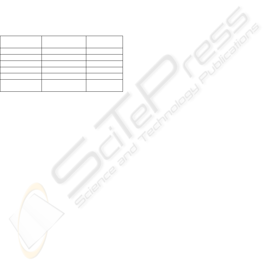
Each of the separate classifiers that compose the

combined classifier was tested individually along

with the combined classifier. The number of

misclassifications compared to the manual

classification was recorded and results are

summarised in Table 1. The results clearly show that

there is significant benefit in combining the different

classifiers.

A quality assessment is made using two

measures:

any

missed

p the probability of missed detection

of an obstacle by any single classifier;

all

missed

p the

misclassification of traversable road by combining

all available classifiers.

The measure of missed detection by any of the

classifiers is

{}

:() ( )

any

missed

pobstacle

prob

classifier H p H traversable

∃∈

⎧

⎫

⎪

⎨

⎬

∃=

⎪

⎩⎭

(7)

Such misclassification for the individual

classifiers was found to be as high as

(95%)

any

missed

p > .

The probability of misclassification of traversable

points

all

missed

p when combining all classifiers is

{}

:() ( )

all

missed

p traversable

prob

classifier H p H obstacle

∀∈

⎧

⎫

⎪

⎨

⎬

∀=

⎪

⎩⎭

(8)

The misclassification for the individual classifiers

was found to be as low as

(5%)

all

missed

p < .

ICINCO 2005 - ROBOTICS AND AUTOMATION

350

The detailed results in Table 1 show that although

raw height, step size, and slope all misclassify

around half the points on their own, they can still

enhance the combined classifier. This is because

they detect different types of obstacles. For

example, raw height only looks at the obstacles

height whereas step size only detects changes in

height. In the Combined (with gap removal)

classifier the 4.4% misclassifications have proven to

be acceptable in practice as often it is just small

parts of the road which are mislabelled as obstacles

(the robot simply navigates around the suspicious

terrain).

Table 1: Experimental results from the classifiers

Classifier Misclassifications Percentage

misclassified

Raw height 2334 64.8%

Step size 2156 59.9%

Slope 1657 46.0%

Roughness 663 18.4%

Combined 393 10.9%

Combined (with

gap removal)

157 4.4%

4 SUMMARY

A classifier fusion algorithm was proposed that

enable a mobile robot to locate and travel along a

safe path in a natural environment using a 2D laser

scanner, a civil GPS receiver and odometry.

Although performance of individual classifiers,

based on simple single scan statistics, was not

impressive, the combined set of classifiers were

found to perform quite accetably in classifying a dirt

road from surrounding terrain with less than 5% of

scanned points being misclassified. The performance

was documented in a natural environment. This

work has shown that 2D laser scans can give

considerable information about a semi-structured

natural environment.

Ongoing work includes maintaining an estimate

of the roads position across the trajectory of multiple

robot positions and using this information in the

classifier. Also, quantifying the accuracy of a given

classification without ground truth is being looked

into. Lastly, attempts are being made to detect the

type of road surface currently being navigated on.

This may allow for adaptive tuning of classifiers by

making the thresholds in the hypothesis tests

dependant on the road surface.

REFERENCES

Vandapel, N., 2004. Natural terrain classification using

3D ladar data. 2004 IEEE Int. Conf. On Robotics and

Automation, pp 5117-5122.

Macedo, J., Matthies, L., Manduchi, R., 2000. Ladar-

based Discrimination of Grass from Obstacles for

Autonomous Navigation. Proc. ISER 2000, USA pp

111-120.

Montemerlo, M., Thrun, S., 2004. A Multi-Resolution

Pyramid for Outdoor Robot Terrain Perception, Proc.

AAAI, pp 464-469.

Wettergreen, D., P. Tompkins, C. Urmson, M. D. Wagner

W. L. Whittaker, 2005. Sun-synchronous Robotic

Exploration: Technical Description and Field

Experimentation. Int. Joural of Robotrics Research, vol

24 (1), pp 3-30.

Iagnemma, K., Brooks, C., Dubowsky, S., 2004. Visual,

Tactile, and Vibration-Based Terrain Analysis for

Planetary Rovers. Proc. IEEE Aerospace Conference,

2004, pp 841-848.

Wallace, R., Matsuzaki, K., Goto, Y., Crisman, J., Webb,

J., Kanade, T., 1986. Progress in Robot Road-

Following. Int. Conference on Robotics and

Automation, 1986, pp 1615-1621.

Jochem, T., Pomerleau, D., Thorpe, C., 1993. MANIAC:

A next generation neurally based autonomous road

follower. Proc. of the Int. Conference on IAS-3, pp

592-601.

Bertozzi, M., Broggi, A., 1997. Vision-based vehicle

guidance. IEEE Computer, vol. 30, pp. 49-55, July

1997.

TERRAIN CLASSIFICATION FOR OUTDOOR AUTONOMOUS ROBOTS USING SINGLE 2D LASER SCANS -

Robot perception for dirt road navigation

351

(a)

−4 −3 −2 −1 0 1 2 3

)

(c)

(d) (e) (f)

Figure 2: Results of different terrain classifiers on a single laser scan (Y-axis is up and the X-axis increases to the

right). A photograph shows roughly where the robot was standing. A double arrow shows how the road in the

hotograph corresponds to its location in the laser scan. The labels are (a) raw height, (b) step size, (c) slope, (d)

roughness, (e) combined, and (f) combined with gap removal. Red points represent obstacles and green

oints the

traversable terrain

ICINCO 2005 - ROBOTICS AND AUTOMATION

352