LOCALIZATION FOR A CAR-LIKE MOBILE ROBOT USING
NONLINEAR DYNAMIC MODEL
Niramon Ruangpayoongsak, Hubert Roth and Robert Mayr
Institute of Automatic Control Engineering, University of Siegen, Hoelderinstr. 3, D-57068 Siegen, Germany
Keywords: Localization, Mobile robotics, Kalman filter, Dynamic model.
Abstract: The problem of localization is well known in mobile robotics. A solution is to use a model-based technique
such as a kalman filter with multi sensor data fusion. For a car-like mobile robot, the nonlinear dynamic
model is suitable for robot movement representation. This work presents the discrete extended kalman filter
including a nonlinear dynamic model for the mobile robot localization. As inputs for the kalman filtering,
gyroscope and compass sensors provide the relative and absolute yaw angles. The experiments are
performed on several path types and the averages of the final position errors and the final heading errors are
proposed.
1 INTRODUCTION
The localization problem is a well known important
problem in mobile robotics. No matter how the
environment is or how the functionalities of the
robot are, whether the robot navigates autonomously
or semi-autonomously, it is useful to know where
the robot is. The mobile robot localization can be
classified into two main categories that are relative
(local) localization and absolute (global) localization
as described in (Goel et.al., 1999).
For large scale outdoor environment, the
positioning resolution is effective to have absolute
localization regarding disturbances resulting from a
missing smoothness of the ground surface. The
absolute positioning sensors such as global
positioning system (GPS), differential GPS, beacon
system, natural landmarks are exploited with the
relative positioning sensors e.g. gyroscope to obtain
accurate robot position. On the other hand, in indoor
environment with a smooth and flat surface, the
disturbance is small. However, the satellite signals in
buildings with many walls often fail regarding to
weakness and blindness. Therefore, a good
performance of at least relative localization is
necessary.
Sensors used for relative positioning are e.g.
odometer, compass and gyroscope. These sensors
have different strength and weakness (Nehmzow,
2003). Odometer is a common device used to
provide travelled distances. The relative position
provided by odometers has sometimes an
accumulated error from wheel slippage. The
gyroscope and compass sensors provide the yaw
angle. The gyroscope measures angular velocity.
The integration of this signal provides the relative
yaw angle. The gyroscope has a drift in
measurement. The compass sensor provides the
ready-to-use absolute yaw angle.
The robot’s nonlinear dynamic model realization
and the robot localization using discrete extended
kalman filter is proposed. The comparison of the real
robot position and heading errors by using odometer,
gyroscope, and compass sensor are presented.
This paper is organized as follows: Section 2
explains the robot modelling, section 3 describes the
extended kalman filter, section 4 shows the
calculation of robot estimated positions and
headings, section 5 presents the experimental results
while section 6 contains the conclusion.
2 ROBOT MODELLING
The first step in model based localization is to
develop a suitable mathematical model for the robot.
When considering the structure of the mobile robot,
it is a four wheel vehicle with the driving principle
of a car, steering the front wheels and propelling the
rear wheels. The nonlinear dynamic model
367
Ruangpayoongsak N., Roth H. and Mayr R. (2005).
LOCALIZATION FOR A CAR-LIKE MOBILE ROBOT USING NONLINEAR DYNAMIC MODEL.
In Proceedings of the Second International Conference on Informatics in Control, Automation and Robotics - Robotics and Automation, pages 367-372
DOI: 10.5220/0001176803670372
Copyright
c
SciTePress

represents the dynamic movement of the robot with
the nonlinear characteristics of the side force at the
wheels. This property has majority effect when the
car moves along curvature path. In the following, the
nonlinear dynamic model is introduced and
subsequently the application on the mobile robot is
described.
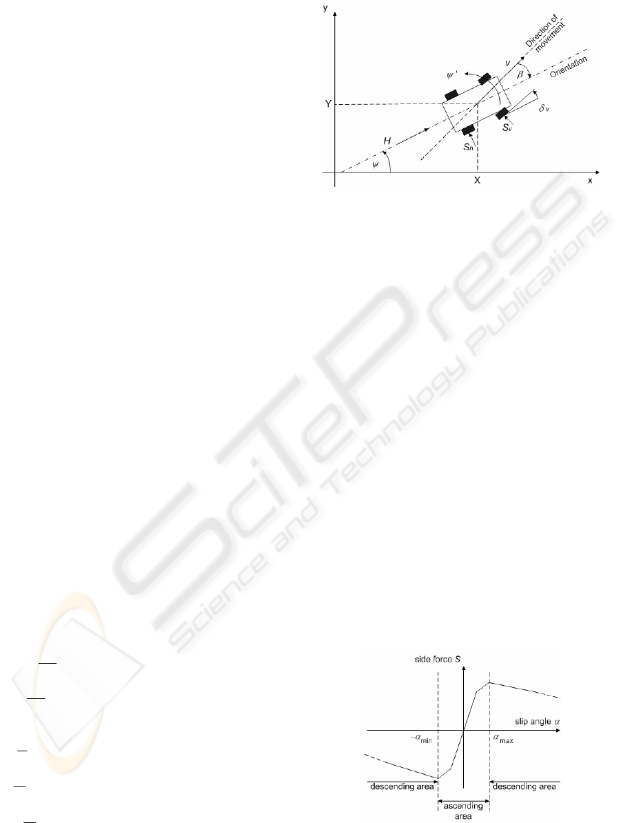
Figure 1: Dynamical variables of the vehicle
2.1 Nonlinear dynamic model
The nonlinear dynamic mathematical model for a
four wheel vehicle was determined as a single track
model describing transverse and longitudinal
dynamics, neglecting roll and pitch angles and
comprising front and rear wheels to one fictitious
wheel (Riekert and Schunck, 1940, Mayr, 1991).
Fig. 1 shows the dynamic variables of a vehicle
as follows:
• the yaw angle
ψ
, vehicle orientation,
• the yaw velocity
ψ
’, the first derivative of the
yaw angle,
• the longitudinal velocity v,
• the sideslip angle
β
,
• the actual position X and Y of the center of
gravity in Cartesian coordinates,
• the front side force S
v
and the rear side force
S
h
,
• the rear longitudinal forces H resulting from
the driving motor,
• the steering angle
δ
v
.
In addition, there are the following constants:
Vehicle mass m, moment of inertia
θ
and the
distances l
v
(l
h
) between the front (rear) wheels and
the longitudinal axes of the car.
Based on the balance of the forces acting on the
vehicle in the longitudinal and lateral directions, the
torques and the kinematic conditions, the nonlinear
dynamic vehicle model is presented as follows:
(){}
ββψβ
cossin
1
h
STH
mv
+−−=
&
&
(){}
δβ
+− cos
1
v
S
m
v
(1)
ψ
ψ
′
=
&
(2)
()
hhvv
lSlS −=
δ
θ
ψ
cos
1
&&
(3)
(){}
ββ
sincos
1
h
STH
m
v −−=
&
(){}
δβ
+− sin
1
v
S
m
(4)
The front and rear side forces S
v
and S
h
of the
vehicle depend on the slip angles
α
v
and
α
h
, while
α
v
depends itself also on the steering angle
δ
v
. The
nonlinear functions Γ
v
and Γ
h
determine the
dynamics in the tires as follows:
)(
vvv
S
α
Γ
=
(5)
)(
hhh
S
α
Γ
=
(6)
By these functions representing a characteristic
line, the behavior of the wheels and the tires is taken
into consideration. This characteristic line includes
limitations and descending behavior for high values
in the argument. As shown in Fig. 2, here the
functions are approximated by three straight lines
describing the dependence of side force values S on
their argument
α
. For low arguments, a nearly
proportional ascend of the side force can be
recognized, while beyond the value
α
max
the side
force is descending. At
α
max
the value for the
corresponding side force reaches its maximum. The
area below
α
max
is called the ascending part, while
the area, where the side force descends is called the
descending part of the characteristic line. As a
Figure 2: Characteristic line Γ of the wheels and tyres
ICINCO 2005 - ROBOTICS AND AUTOMATION
368

consequence of the gradual inverse dynamics, the
car would begin to skid when driving in the
descending part. During a normal maneuver without
skidding, every wheel of the vehicle is working in
the ascending area of the characteristic line. This
nonlinear characteristic coming from automotive
technology is also applicable to a car-like mobile
robot in indoor environment over dry and flat floor.
As here, high absolute values for
α
v
and
α
h
will
never come up, the functions Γ
v
and Γ
h
can be
simplified to the amplification factors c
v
and c
h
.
Then, (5) and (6) result in
⎟
⎠
⎞
⎜
⎝
⎛
+−==
δψβα
&
v
l
ccS
v
vvvv
(7)
⎟
⎠
⎞
⎜
⎝
⎛
+==
ψβα
&
v
l
ccS
h
hhhh
(8)
2.2 Model realization
The mobile experimental robot for locomotion and
intelligent navigation (MERLIN) has been designed
and developed for both, indoor and outdoor
environments. The sensors onboard are odometer,
gyroscope, 3D compass, ultrasonic sensor, infrared
sensor, and bumper as shown in Fig. 3. The semi-
autonomous tele-control using joystick and path
commands are available via internet (Kuhle et. al.,
2004).
The moment of inertia from calculation is equal
to 0.169167 kg·m
2
. The side force constants c
v
and
c
h
are from experiments. By keeping a constant
steering angle
δ
v
and a constant driving motor force
H, the robot drives on a circular path with a constant
speed and the robots position is externally recorded
by a V-scope
TM
positioning sensor. The data are
exploited with the model equations to obtain the side
force constant. The results are c
v
= 168450 and c
h
=
152290. The length from the center of gravity to the
front wheels is l
v
= 0.15 meter and to the rear wheels
l
h
= 0.15 meter. The mass of the robot is m = 7 kg
including the batteries. Due to the surface of the
robot is small and as the robot drives with low
speed, the air resistance is neglected.
3 EXTENDED KALMAN FILTER
(EKF)
The kalman filter is a model-based sensor fusion
technique. Two main processes are time update and
measurement update. For a nonlinear dynamic
system, the discrete extended kalman filter is applied
(
Brown, 1983, Welch and Bishop, 2002). Assume
that a nonlinear process has a state vector
and
is governed by the non-linear stochastic differential
equation with a measurement
that is
n
x ℜ∈
m
z ℜ∈
x
k
= f (x
k-1
,u
k-1
,w
k-1
), (9)
z
k
= h(x
k
, v
k
), (10)
where w
k
and v
k
represent the process and
measurement noise. After linearization, the
linearized state transition matrix is represented
without noises. The Jacobian matrix of the partial
derivatives of f with respect to x is
[]
[]
[]
)0,,
ˆ
(
1, kk
j
i
ji
ux
x
f
A
−
∂
∂
=
,
(11)
where the state vector x is
T
vx ][
ψψβ
′
=
,
(12)
and the Jacobian matrix of partial derivatives of h
with respect to x is
Figure 3: MERLIN
[]
[]
[]
)0,
~
(
, k
j
i
ji
x
x
h
H
∂
∂
=
,
(13)
where h is
T
xxxxh ][
4321
=
.
(14)
The kalman filtering process starts from
initialization of all state variables and matrices.
Assume that the process and measurement noises are
Gaussian with zero mean and are constant
throughout the process. The priori estimate state
variable
and the priori estimate error covariance
at time step k are
−
k
x
ˆ
−
k
P
LOCALIZATION FOR A CAR-LIKE MOBILE ROBOT USING NONLINEAR DYNAMIC MODEL
369

Figure 4: Architecture of the robot localization system
)0,,
ˆ
(
ˆ
1 kkk
uxfx
−
−
=
,
(15)
QAPAP
T
kkkk
+=
−
−
1
,
(16)
where Q is the process noise constant matrix. After
that the kalman gain K
k
, the posteriori estimate state
variable
, and the posteriori estimate error
covariance P
k
x
ˆ
k
are calculated as follows:
1
)(
−−−
+= RHPHHPK
T
kkk
T
kkk
,
(17)
))0,
ˆ
((
ˆˆ
−−
−+=
kkkkk
xhzKxx
,
(18)
−
−=
kkkk
PHKIP )(
,
(19)
where R is the measurement noise covariance.
The inputs of the robot model are the steering
angle
δ
and the driving motor force H. Let the input
vector at time step k be
u
k
= [
δ
k
Η
k
]
T
,
(20)
and let the measurement vector be
z
k
= [z
β,
k
z
ψ,
k
z
ψ
’,k
z
v,k
]
T
,
(21)
where z
β,
k
, z
ψ,
k
, z
ψ
’,k
, and z
v,k
are the measured values
of the state variables at time step k. As the robot
drives very slow and, thus, the sideslip angle, which
is difficult to sense, is of minor importance, the
measurement value of the sideslip is set to zero for
all time steps k. Regarding the system model in (1–
4), the discrete system is first obtained using Euler’s
method (
Franklin, 1998). The process and
measurement noise covariance matrices Q and R are
tuned off-line in the simulation for appropriate value
and kept constant during the iterative process. The
selected values are 1x10
-6
for all diagonal matrix
elements.
Figure 5: Variables based on odometer (cont.)
4 POSITION AND HEADING
CALCULATIONS
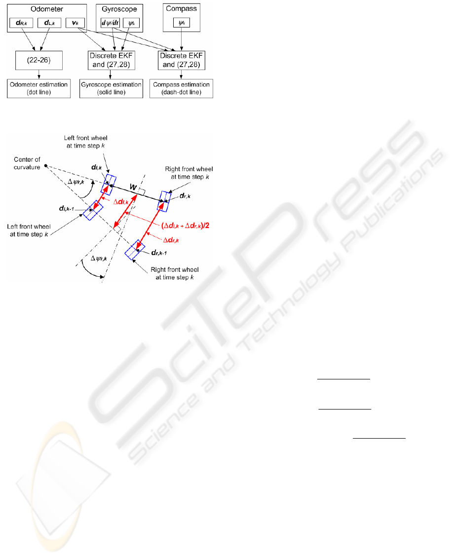
As shown in Fig. 4, three different estimated paths
are from using measurement of odometer,
gyroscope, and compass estimation. The odometer
estimated position and heading is the non-model
based whereas the other two estimations are based
on kalman filter and the nonlinear dynamic model.
4.1 Odometer position and heading
estimation
The position x
odo,k
, y
odo,k
and heading
ψ
odo,k
at step k
are calculated from
kodo
kLkR
kodokodo
dd
xx
,
,,
1,,
cos
2
ψ
⎟
⎟
⎠
⎞
⎜
⎜
⎝
⎛
∆+∆
+=
−
,
(22)
kodo
kLkR
kodokodo
dd
yy
,
,,
1,,
sin
2
ψ
⎟
⎟
⎠
⎞
⎜
⎜
⎝
⎛
∆+∆
+=
−
,
(23)
⎟
⎟
⎠
⎞
⎜
⎜
⎝
⎛
∆−∆
+=
−
−
W
dd
kLkR
kodokodo
,,
1
1,,
tan
ψ
ψ
,
(24)
1,,, −
−
=
∆
kRkRkR
ddd
,
(25)
1,,, −
−
=
∆
kLkLkL
ddd
(26)
where ∆d
R,k
is the difference of driven distances of
the right wheel between the time steps k and k-1 as
shown in Fig. 5. Note that similar calculation is
applied to the difference of distances left ∆d
L,k
. Here,
d
L,k
represents the already driven distance of the left
wheel at time step k, while d
R,k
is the driven distance
of the right wheel. These driven distances since the
beginning of the ride can be computed from the
amount of pulses from the odometer on each wheel.
The wheel base W is the distance between the center
ICINCO 2005 - ROBOTICS AND AUTOMATION
370

of the left wheel to the center of the right wheel and
is equal to 23.5 cm.
4.2 Position and heading estimation
using gyroscope and compass
The estimated positions of the relative yaw angle of
the gyroscope and absolute yaw angle of the
compass are calculated by using
()
1
cos
−
+
−
⋅=
kkkkk
xvstx
β
ψ
,
(27)
()
1
sin
−
+
−
⋅=
kkkkk
yvsty
β
ψ
,
(28)
where v
k
,
ψ
k
, and
β
k
are posterior estimated state
variables as in (18). The estimated robot heading is
ψ
k
. st is the time step. Here also the kalman filtering
is applied.
5 EXPERIMENTAL RESULTS
The experiments were performed in indoor and the
sensor data were collected for off-line plots using
MATLAB. All graphs scale has unit in meter and
the data sampling rate is 0.2 sec. The test is designed
for testing the performance of localization when the
robot moves straight on, in a curve path, and the
combination of both.
5.1 Test results
As already mentioned, in order to improve the
quality of the measurement signals, the data coming
from the gyroscope as well as the data from the
compass was subsequently processed by the kalman
filter using the measured velocity signal from the
odometer.
Odometer: Please note that for comparison, the
data coming from the odometer itself (dot line) is
plotted directly using (22-26) and, thus, not updated
by the kalman filter. Due to (24), (25) and (26),
relevant odometer data is not only the average of the
wheel movements but also the difference of the
movements of the left and right wheel in order to get
information about the change of orientation of the
robot.
Gyroscope: The measured yaw angle by
gyroscope are applied as inputs to kalman filter
measurement updates and the positions are obtained
from (27) and (28) shown as solid line. Please note,
that here the odometer only provides the
measurement value for the velocity.
Compass: Similarly, by using the compass yaw
angle with kalman filter, the position estimation
from (27) and (28) are represented by dash-dot line.
Please note, that here also the odometer only
provides the measurement value for the velocity.
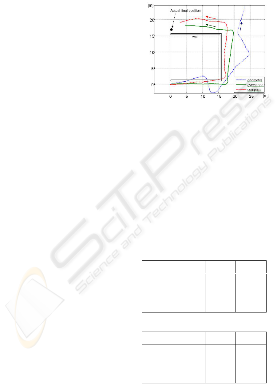
Figure 6: Wall-path estimated positions
The wall-path is shown in Fig. 6. At the wall
corners, the robot turns with minimum radius curve.
The estimated final position using odometer has
sometimes large error as shown in the figure. The
gyroscope has drift in some trials whereas the
compass result is quite static for all trials with error
of deviation in measurement as in line path.
For every path type, several driving tests were
performed. Regarding each driving test, the real final
position determined was compared to the position
value measured by the on-board sensors and the
resulting errors were calculated. Subsequently, the
Table 1: Average position errors (e
pos
)
Odometer
(meters)
Compass
(meters)
Gyroscope
(meters)
Rectangular 0.71 0.33
0.17
U 0.88 0.38
0.12
Arcs
0.26
0.32 0.29
Line1 0.53
0.27
1.02
Line2
0.19
0.78 0.27
Wall 15.09
3.35
5.44
Table 2: Average heading errors (e
heading
)
Odometer
(degrees)
Compass
(degrees)
Gyroscope
(degrees)
Rectangular -23 14
-1
U 7 12
2
Arcs 6 110
1
Line1
5
61 6
Line2 5 -91
0
Wall -58 -52
-10
LOCALIZATION FOR A CAR-LIKE MOBILE ROBOT USING NONLINEAR DYNAMIC MODEL
371

average error values result from the averages of the
respective errors of all similar driving tests.
The average errors in position and heading are
summarized in Tables 1 and 2, respectively. The
position error e
pos
is the error between the actual
final position and the estimated final position. Based
on the actual and estimated values for the yaw angle,
the heading error e
heading
is the error of robot heading
at the final position. These errors are calculated by
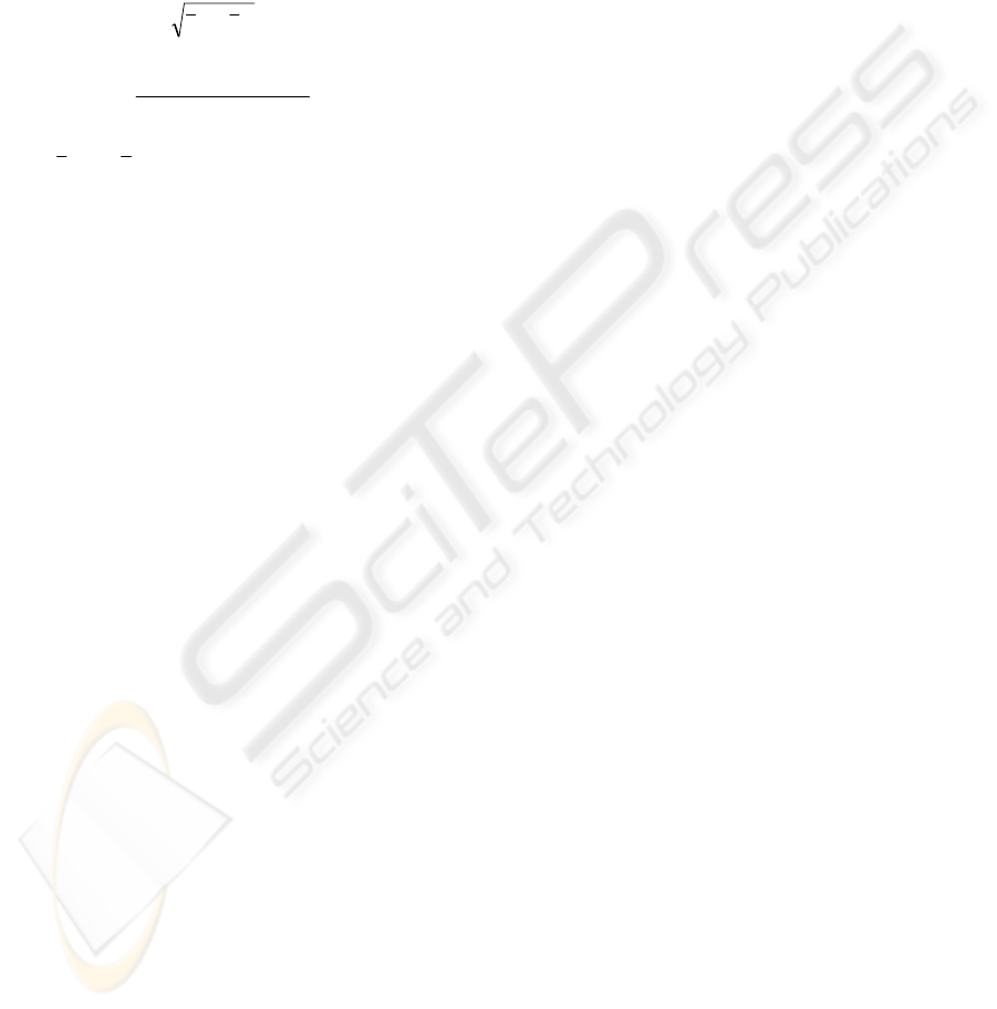
22
yxpos
eee +=
,
(29)
()
n
e
n
i
iactualiestimate
heading
∑
=
−
=
1
,,
ψψ
,
(30)
Where
x
e
and
y
e
are the mean of error in x and y
direction from several driving tests.
ψ
estimate,i
and
ψ
actual,i
are the estimated and actual final heading of
test number i, respectively.
In Table 1, the average of final position errors of
gyroscope are not the largest in all trajectories. Due
to the localization based on model, the position
errors of compass and gyro are not much different.
The gyro and compass with discrete EKF
outperforms the odometer positioning for wall path.
As in Table 2, the average of final heading errors of
the well calibrated gyroscope present the excellent
performance over compass and odometer.
5.2 Discussions
For the line1 path, both average position and
heading errors of gyroscope are larger than those of
odometer and compass. This presents the minority
performance of the gyroscope over the odometer in
line1 path by the mechanical structure of the robot.
For the trajectories containing arcs path that are
rectangular, U, and arcs path, the yaw angle
measurement dominates in the position estimation
process. The well calibrated gyroscope presents
good performance without drift. Nevertheless, for
the large scale scenario as for wall path, the
gyroscope provides good estimation, because here
the drift is not relevant.
The compass yaw angle deviation occurs in all
trajectories. This error shows up in most of all the
driving tests. The average errors of final heading for
all trajectories in Table 2 are in most cases larger.
However, there are some cases that the deviation
doesn’t exist as shown in Fig. 6.
For the odometer estimated position, the large
error is presented in the wall path. This error is
caused by the slippage in the wheels and does not
always occur in all driving tests. However, the final
position and heading errors are larger than those of
the gyroscope, except in line1 and line2 trajectories
regarding to the previous discussion of the error in
the estimation using gyroscope.
6 CONCLUSIONS
The discrete extended kalman filter is applied to a
car-like mobile robot for improvement of
localization using the nonlinear dynamic model. The
experiments are performed on six path types and the
final position error and final heading error using
odometer, gyroscope, and compass data are
compared. The well calibrated gyroscope provides
minority performance in robot final position for
line1 path. For the other five path types, the
gyroscope position errors are smaller than those of
odometer and the in performance in final heading of
the gyroscope dominates the compass and odometer
for all trajectories.
REFERENCES
Brown, R.G., 1983. Introduction to random signal
analysis and kalman filtering, John Wiley & Sons,
USA, p. 300.
Franklin, G. F., Powell, J. D., and Workman, M., 1998.
Digital Control of Dynamic Systems, 3
rd
edition,
Addison Wesley Longman, p. 59.
Goel, P. and Roumeliotis, S. I. and Sukhatme, G. S., 1999.
Robot Localization Using Relative and Absolute
Position Estimates In Proc. 1999 IEEE/RSJ
International Conference on Intelligent Robots and
Systems, Kyongju, Korea, Oct. 17-21, pp. 1134-1140.
Kuhle, J., Roth, H., Ruangpayoongsak, N., 2004.
MOBILE ROBOTS and airships in a multi-robot
team. The 1st IFAC Symposium on Telematics
Applications in Automation and Robotics, Helsinki
University of Technology, Finland, pp. 67-72.
Mayr, R., 1991. Verfahren zur Bahnfolgeregelung für ein
automatisch geführtes Fahrzeug, Dissertation,
University of Dortmund, Dortmund, Germany.
Nehmzow, U., 2003. Mobile Robotics: A Practical
Introduction, 2
nd
Edition, Springer-Verlag, London.
Riekert, P. and Schunck, T.E., 1940. Zur Fahrmechanik
des gummibereiften Kraftfahrzeugs. Ing. Arch., Vol.
XI, pp. 210-224.
TWelch, G., and Bishop, G., 2002. An Introduction to the
Kalman Filter, UNC-Chapel Hill, USA, TR 95-041.T
ICINCO 2005 - ROBOTICS AND AUTOMATION
372
