Efﬁcient Gridding

of Real Microarray Images

Giuseppe Lipori

Dipartimento di Scienze dell’Informazione

Universit

a degli Studi di Milano

Via Comelico, 39/41 - 20135 Milano

Work partially supported by the PASCAL Network of Excellence under EC grant no. 506778.

Abstract. DNA microarrays technology is very recent and rapidly evolving. At

present, it is widely used in the analysis of gene expression. The interpretation of

the data crucially depends on the accuracy of the localization of the circular spots,

which are placed in rectangular grids. The problem is complicated by the presence

of many local deformations of the grid, by the high variability in luminance of

the spots, by noise and other disturbances due to the biological nature of the

experiments. In this paper we implement an automatic method for the gridding of

real microarrays that takes into account most of the open problems by exploiting a

recently introduced image transform, the Orientation Matching Transform, which

enhances circular patterns of a speciﬁc size.

1 Introduction

DNA microarray consists of a solid surface onto which DNA molecules have been

chemically bonded. Microarrays are widely used to study gene expression in order to

associate gene activities with biological processes and to group genes into networks of

interconnected activities. They are very advantageous since they allow to measure the

expression of thousands of genes in parallel and in a quasi automated way. On the other

hand every microarray experiment poses the problem to handle and analyze a huge mass

of data, which is often corrupted by noise or some other disturbances.

A common type of microarray is called pin spotted because it is produced via a

robotic arm that spots the DNA probes on the microscope slides. The robot is shaped as

a grid of pins and so a typical spotted microarray is composed of a set of regular grids of

circular spots, as schematized in Figure 1. This is the type of microarrays on which we

will focus and when we speak of microarrays we really intend pin spotted microarrays.

For a full explanation of how microarrays are engineered and for a survey of all types

of existing technologies refer to [11].

The result of a microarray experiment is presented in the form of an image, where

the most expressed genes are indicated by high intensity spots. The ﬁrst stage of the

analysis is called gridding, that is the process of assigning coordinates to the spot lo-

cations. Then the data is segmented in order to separate the foreground pixels from

the background. Finally comes the intensity extraction that corresponds to reading the

intensity of expression of each spot.

Lipori G. (2005).

Efﬁcient Gridding of Real Microarray Images.

In Proceedings of the 1st International Workshop on Biosignal Processing and Classiﬁcation, pages 121-130

DOI: 10.5220/0001192501210130

 SciTePress

Fig.1. The structure of a microarray and the image axes vs. the grid axes.

We will limit the analysis to the gridding, which is a crucial phase as the accuracy of

the whole analysis depends on the precision with which spots are located. Sometimes

the problem of gridding is solved by requiring human intervention to specify some

points in the grid or even to register individual spots. This article aims at automatizing

the gridding task as much as possible via the application of a deformable gridding

proposed in [2] and then developed in [3], [4]. The method is based on the Orientation

Matching Transform (OMT) presented in [5] and until now it has been evaluated solely

on synthetic images generated for the purpose. The contribution of this paper is the

adaptation of the technique to make it suitable and robust for the treatment of real

images of microarrays that present much more difﬁculty to the gridding.

2 Gridding

Both the number of grids on a slide and the number of spots within a grid may vary

in different microarrays. In general the space between the grids is much larger than the

space between the spots and this suggests to treat each grid separately. An example of

a good quality microarray grid is shown in Figure 2.

The biological nature of the data makes it prone to a number of problematic situa-

tions that make gridding a difﬁcult task: high background noise, irregular shape or size

of the spots, presence of faint spots, imperfect alignment of the spots along the rows

or columns of the grid, local deformations as well as small rotations of the grid due to

wrong placement under the image scanner, sensible skew of the two axes and so on. All

these issues need to be treated automatically in order to locate the spots in an accurate

way. However most of the approaches so far presented for microarray gridding, e.g. [1]

and [8], try to pose some restrictions on the data or make strong assumptions, such as

requiring grid rows and columns perfectly aligned along the x and y axes of the image.

In our approach we assume the axes of the grid free to rotate with respect to the

axes of the image (see Figure 1). In particular the row axis X

′

can make an angle

α <

with the horizontal axis X of the image, and the column axis Y

′

can make

with X

′

an angle β − α 6=

. Moreover, we will allow the spacings (∆x, ∆y) of the

122

Fig.2. A good quality grid and its OMT (with parameters r = 2, R = 4)

spots (along the columns and the rows respectively) to be different, and we assume no

a priori knowledge on the number of rows and columns.

The strategy of the gridding is divided into the following, successive steps:

– OMT: transform of the image to enhance the circular objects of a speciﬁed size;

– regular grid: use of the Radon Transform (RT) to project the OMT output along

all directions in order to identify the axes’ angles α and β; the knowledge on an-

gles enables us to determine the grid spacings and the coordinates of the ﬁrst spot

, y

); the tuple (α, β, ∆x, ∆y, x

, y

) completely speciﬁes the regular grid po-

sitions (x

, y

)

= x

+ i∆y cos β + j∆x cos α

= y

+ i∆y sin β + j∆x sin α (1)

that best match the actual microarray grid;

– deformable grid: deformation of the regular grid by adopting a Bayesian approach:

choice of the trade off between regularity and accuracy of superposition on the

actual spots, calculated via a Maximum A Posteriori (MAP) scheme.

2.1 Orientation Matching Transform

The OMT is an extension of the Hough Transform for circles and was ﬁrst proposed

in [5]. Our scope here is to accurately segment the spots from the background. Two

common approaches to the problem would be to work on the edge image or to threshold

the gray scale image according to some criteria. Both these strategies suffer from many

complications due to the high variability of spot luminance, to the presence of noise and

in particular to the existence of many spots that are almost as dark as the background.

The OMT presents the sure advantage that it does not work on the absolute luminance

of the spots and it is essentially invariant to contrast changes.

In details, let A

(0, 0) be the annulus of radii r and R centered in the origin, that is

(0, 0) =



(x, y) ∈ R | r ≤ x

+ y

≤ R



123

If we deﬁne φ

∗

in such a way that

cos φ

∗

(x, y) =

+ y

; sin φ

∗

(x, y) =

+ y

and if φ(x, y) is the orientation of the image gradient in (x, y), then the OMT is given

OM(u, v) =

π(R

− r

)

(u,v)

cos (φ

∗

(x − u, y − v) − φ(x, y)) dx dy (2)

The factor

π (R

−r

)

is equal to the inverse of the area of the annulus A

(u, v); it works

as a normalization factor to obtain −1 ≤ OM (u, v) ≤ 1. In words, (2) uses the cosine

to measure the similarity between the orientation φ

∗

of the gradient of ideal circles

centered in (u, v) (with radii ranging in [r,R]) and the orientation of the image gradient

around the same point. It is sufﬁcient to know the range of radii of the spots in a certain

microarray to apply the correct transform

Figure 2 shows the output of the OMT for the sample image; notice how the faint

spots are partially recovered in the transform image.

Since cos(φ

∗

− φ) = sin φ

∗

sin φ + cos φ

∗

cos φ, the OMT can be implemented

as the sum of two image ﬁlterings, which is computationally much more efﬁcient than

applying the deﬁnition as it is.

2.2 Radon Transform projections

The Radon Transform [9] is at the basis of Computer Tomography because it permits

to reconstruct an unknown 2-dimensional function (typically the image of a slice of

biological tissue) by calculating its integral along all lines passing through it in all

possible directions. In our context we do not need the inverse transform, what we need

is to identify the direction of the axes X

′

and Y

′

of the grid. We do it by analyzing the

projections of the OMT image over different orientations.

The formal deﬁnition of the 2D RT of a signal f is

s,φ

(f) =

∞

−∞

∞

−∞

f(x, y)δ(x cos φ + y sin φ − s) dx dy (3)

where the Kronecker delta is used to specify the line of integration deﬁned in polar

coordinates (s, φ).

Our deﬁnition is equivalent to the original

O M (u, v) =

2π(R − r)

(u,v)

cos (φ

∗

(x − u, y − v) − φ(x, y))

(x − u)

+ (y − v

)

dx dy

as both exhibit the desired property of normalization (they are both dimensionless).

Usually the right parameters r and R remain fairly constant across experiments made on the

same type of support. However they can vary very much from microarray to microarray and it

is crucial to choose a good couple of radii for the gridding to work.

124

If I is the gray scale image of the grid, we are interested in the function

(I) =

s,φ

(OM(I))| ds (4)

Fig.3. The Radon transform vs. the Γ

peaks

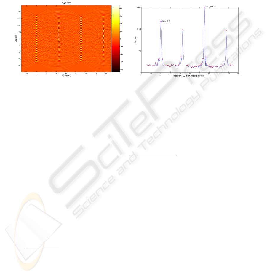
The left side of Figure 3 depicts the output of R

s,φ

(OM(I)) applied to the image in

Figure 2; notice how the projection width shrinks and how the proﬁle gets better deﬁned

as the angle approaches the perfect alignment with an axis of the grid. On the right side

it is shown the behavior of Γ

(I); the main directions of the grid are calculated by

choosing the two peaks that are best correlated according to the criterium

(α, β) = arg max

(φ

,φ

)

(I) · Γ

(I)

1 + | cos(φ

− φ

The two sub-peaks corresponding to the diagonals of the grid are also visible.

The identiﬁcation of α and β allows us to study the row and column structure of

the grid. In principle it would be enough to take R

s,α

(OM(I)) and R

s,β

(OM(I)) over

all s, and to study the two proﬁles separately in order to estimate the number of rows

and columns and the respective spacings (∆

, ∆

). However care must be taken at this

stage of the gridding because the shape of the two projections can pose some problems:

there can be very different peak intensities due to rows/columns with many faint spots

and, above all, false peaks can be caused by dirt found on the slide in between the wells

that contain the spots. Therefore there is need for some processing to normalize the

signals and clean them from possible causes of error.

Differently from [3], in (4) we introduce the absolute value because the integral of

s,φ

(OM (I)) over s is equal along all directions and it is close to zero (recall −1 ≤

O M (u, v) ≤ 1), while the integral of |R

s,φ

(OM (I))| increases with the accentuation of

peaks (w.r.t. valleys) in the projection.

125

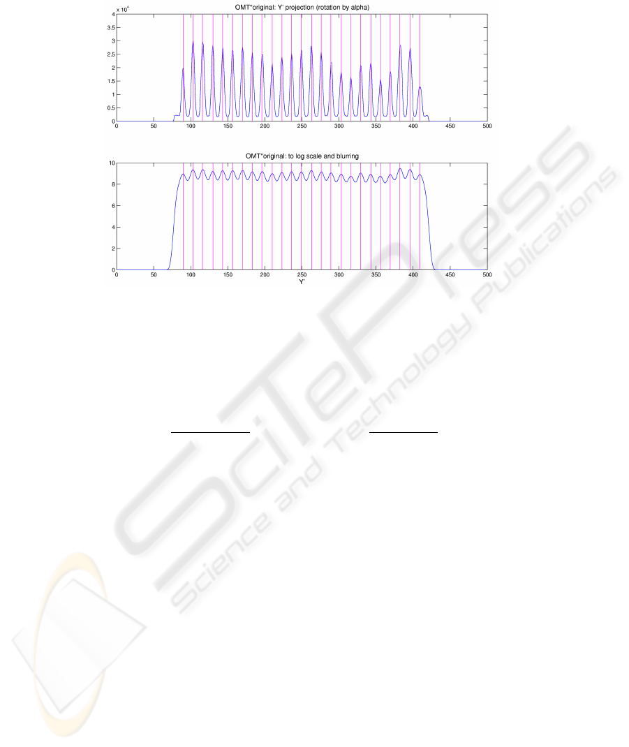
Fig.4. The Y

′

proﬁle corresponding to the projection of the grid transform along angle β (before

and after treatment)

To this end, we experimentally found that it is much more robust to analyze the

proﬁle of a reinforcement of the OMT, that is to use the projections of

s,φ



(1 + OM (I))

· I



, where 0 ≤

1 + OM (I)

≤ 1 .

Afterwards we attenuate the variability in peak intensities by passing to the loga-

rithmic scale and, in order to ﬂatten the false peaks, we apply a Gaussian ﬁltering whose

support size depends on a rough estimate of the peak spacing. See Figure 4 for the Y

′

axis projection (before and after treatment) of the sample image (the X

′

axis projection

is analogous).

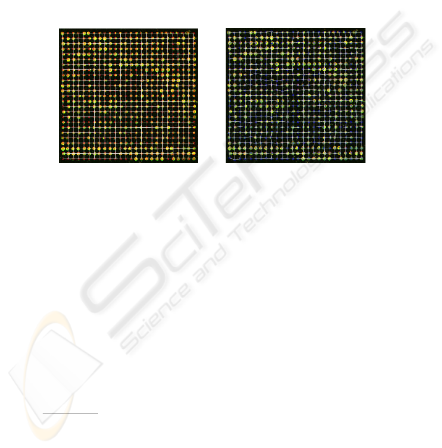
After the individuation of all peaks we use (1) to build the regular grid (Figure 5)

that best overlaps the microarray grid.

2.3 Bayesian gridding

The ﬁnal step of the gridding technique aims at deforming the regular grid in order to

get the best possible match between the spot centers and the grid positions. A possible

solution to this problem is to use a Bayesian scheme of inference, like that proposed in

[7]. This methodology consists in building a model of microarray grids (the so called

prior) and use a Maximum A Posteriori (MAP) approach to establish which is the best

gridding on a given instance of the problem according to that model. In symbols, if I is

the image in input to our system and G is the model of the grid, we want to ﬁnd G that

126

maximizes

P (G|I) =

P (G)P (I|G)

P (I)

∝ P (G)P (I|G) (5)

The choice of the grid model is very important because on one hand its precision im-

proves the quality of the gridding, but on the other hand its richness in details affects

the complexity of the computation of

∗

= arg max

P (G)P (I|G) = arg max

log P (G|I) . (6)

In [7] the model G really describes a grid because it takes into account both the posi-

tions of the spots and the length of the arcs that connect each spot to its neighbors. For

simplicity we follow the analysis of [4], where G is in fact a prior based on 1-cliques:

each spot is treated independently of its neighbors and of the rest of the grid. However,

while they use a computationally expensive and potentially sub-optimal algorithm (the

Simulated Annealing) to solve (6), we exploit the mutual independence of the spots

to ﬁnd the optimal solution in an efﬁcient fashion. If a grid is just a collection of in-

dependent spots, then every spot g

is assumed identically distributed (according to a

Gaussian distribution) around the corresponding position t

of the regular grid. The

joint distribution of G becomes very simple

P (G) ∝ exp





−

− t

i,j

)

−1

− t

i,j

)





The model of G depends only on the variance of the Gaussian distribution, which should

be estimated from a sample of grids. However we assume no mutual dependence of the

Gaussian displacements along the two axes (zero covariance) and we ﬁx

= Σ =



· σ





∆x

∆y



where k is a constant that regulates the amplitude of the spots’ displacement.

The second factor of the objective function is the likelihood that measures how well

the observed instance ﬁts the model. Like in [4] we adopt as observation model

P (I|G) ∝ exp





−

(1 − OM (g

))





that is we estimate the accordance of the model with the observed data by measuring

how close the locations of the deformable grid are to the center of circular objects. It is

clear that the deformation of the regular grid is performed by varying the model G in

order to ﬁnd

∗

= arg max

log P (G|I) = arg max

{log P (I|G) + log P (G)} (7)

by balancing the opposite contributions of the ﬁrst term, which privileges the regularity

of the grid, and the second one, which rewards a good matching of the grid with the real

spots’ positions.

127

It is important to notice that the objective function (7) can be decomposed in a set

of independent sub-problems, each corresponding to a single spot

∗

= arg min



− t

i,j

)

−1

− t

i,j

) + (1 − OM (g

))



and G

∗

can be calculated quite efﬁciently by an exhaustive visit of a small neighborhood

of each t

without implementing a more sophisticated search algorithm. The process

produces the result shown on the right in Figure 5.

Fig.5. The regular grid vs. the deformed grid

3 Experimental results

The experimental evaluation of our gridding technique has been quite difﬁcult to ac-

complish because of the lack of ground truth available on real biological data. However

we wanted to avoid the generation of artiﬁcial microarray grids to test upon, since the

synthetic images do not simulate very effectively all the involved variables: variability

of the spots’ shape, the “texture” of the background and its noise, the presence of imper-

fections due to the unskillfulness of the experimenter and so on. It is sufﬁcient to take a

look at the internet site of the Stanford Microarray Database (SMD) [10] to realize how

heterogeneous microarrays are; this is the consequence of the variety of supports avail-

able combined with the unequal experience of different experimenters, plus the fact that

a single experiment is so expensive that it might not be convenient to repeat it in case

of imperfections.

As a term of comparison we use the gridding done by the software GenePix [6],

which is a sophisticated commercial software very popular among bioinformaticians

GenePix carries out the complete analysis of a microarray plate, from the gridding to the inten-

sity extraction. Unfortunately its speciﬁcations do not give any information on the principles

of its functioning, nor on its computational cost, being it a proprietary software.

128

The SMD makes available many GenePix raw data output ﬁles, which contain the coor-

dinates of the bounding box of each spot, together with the original microarray images.

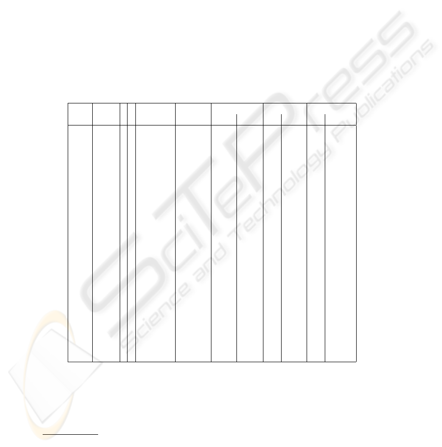
In Table 1 we present the evaluation of our gridding technique given in terms of statis-

tics on the distance between the locations of the deformed grid and the centers of the

bounding boxes, taken as the ground truth of the data. The choice of parameters (r, R)

for each microarray is made by presenting to a human operator the output of the OMT

on a grid chosen at random and over a wide range of possibilities (R ∈ {4, . . . , 10}

and r ∈ {R − 4, . . . , R − 1}), asking for a preference. The best possible choice that

can be made visually is the one that produces the OMT with the brightest and sharpest

peaks in correspondence to the spot locations. The difference R − r decreases with the

regularity of the spots’ size within the grid and, in ideal conditions, the choice should

be such that r = R − 1.

Table 1. Gridding results

ID grids r R grids time per mean angles error: mean error: std dev

size completed grid (sec) α β x y x y

11704 26×26 4 6 11/32 15.8 -0.32

◦

90.43

◦

1.09 1.05 0.87 0.94

14013 31×32 4 5 32/32 19.7 0.02

◦

89.94

◦

0.59 0.60 0.22 0.31

14317 26×26 3 6 3/32 15.5 -0.4

◦

90.1

◦

0.88 0.98 0.72 0.93

15989 18×19 6 8 16/16 13.2 0.59

◦

90.02

◦

0.83 1.12 0.60 1.28

17995 19×19 4 7 16/16 14.8 -0.12

◦

89.89

◦

1.01 1.18 0.80 0.97

19880 20×20 6 7 5/16 15.5 0.68

◦

89.91

◦

1.36 1.67 1.17 1.69

20385 18×18 7 8 36/48 13.3 0.14

◦

91.44

◦

3.98 7.73 6.70 9.48

21635 13×16 6 7 44/48 9.5 -0.51

◦

89.63

◦

1.26 2.44 2.25 3.62

22588 18×16 6 8 9/16 10.1 8.15

◦

98.42

◦

1.13 1.46 0.95 1.53

24047 19×19 7 8 15/16 14.3 0.16

◦

90.08

◦

0.91 1.03 0.89 1.02

24494 17×17 3 6 13/16 11.6 -1.11

◦

89.78

◦

1.28 1.63 1.02 1.83

24753 15×16 3 4 11/32 8.7 0.39

◦

90.1

◦

3.88 1.70 2.86 1.56

25978 30×30 5 6 48/48 19.7 0.20

◦

90.22

◦

0.68 1.05 0.59 0.82

30855 18×18 7 8 16/16 13.0 0.1

◦

89.93

◦

0.82 0.85 0.76 0.71

31784 18×20 5 7 14/32 12.6 -0.09

◦

89.96

◦

1.86 3.45 4.72 6.98

32827 17×17 3 5 16/16 11.4 0.44

◦

90.37

◦

0.89 1.23 0.81 1.04

32898 30×30 4 5 43/48 21.8 -0.1

◦

89.95

◦

0.77 1.57 0.68 1.32

34727 24×24 4 5 4/16 16.0 0.77

◦

90.22

◦

0.99 1.21 0.90 1.15

40380 18×20 5 7 31/32 12.6 0.65

◦

89.63

◦

1.11 1.00 0.91 0.83

4047 22×24 4 5 7/16 14.4 -0.35

◦

89.89

◦

0.92 1.33 0.67 1.53

42420 25×26 5 6 15/16 16.8 -0.17

◦

89.88

◦

2.73 1.68 6.21 1.38

51736 22×22 5 7 48/48 16.3 -0.10

◦

89.89

◦

0.66 1.06 0.61 0.84

Table 1 also reports the experiment ID of each microarray in the SMD and the

average execution time.

Implementation in MATLAB on a Pentium 4 (3.2 GHz) machine.

129

4 Discussion and conclusion

Our method automatically detects failure of the gridding, which is often due to inputs

whose structure does not match the expected logical structure of Figure 1. For instance

there are frequent situations

in which a correct gridding can never be obtained with

our technique because one or more rows are systematically missing at the bottom of

the grids (due to irrelevant expression of the corresponding genes), so preventing any

possible solution solely based on the data. This is a problem speciﬁc to the context of

microarrays that is not sufﬁciently taken into account by the general method.

In the remaining cases

the gridding works very well as both the error mean and

standard deviation often kept around one pixel, which is desirable and comparable to

the results achieved in [4] over synthetic images

In our experience, the prominent cause of failure is the incorrect evaluation of the

number and position of rows/columns, which results in the automatic discard of the

gridding. Probably it would be enough to require human intervention for the introduc-

tion of the correct number of rows/columns

to achieve a much better performance on

most experiments. In our future work we intend to examine this variant.

References

1. J Angulo and J Serra. Automatic Analysis of DNA Microarray Images using Mathematical

Morphology. Bioinformatics, 19(5):553–562, 2003.

2. G Antoniol and M Ceccarelli. A Markov Random Field Approach to Microarray Image

Gridding. Proceedings of the IEEE International Conference on Pattern Recognition, 2004.

3. G Antoniol, M Ceccarelli, and A Petrosino. Microarray Image Addressing Based on the

Radon Transform. Proceedings of the IEEE International Conference on Image Processing,

2005.

4. M Ceccarelli and G Antoniol. A Deformable Grid Matching Approach for Microarray Im-

ages. Technical report at the Research Center on Software Technologies (RCOST), 2005.

5. M Ceccarelli and A Petrosino. The Orientation Matching Transform Approach to Circu-

lar Object Detection. Proceedings of IEEE International Conference on Image Processing,

pages 712–715, 2001.

6. GenePix Pro. Software for Microarray Image Analysis by Axon Instruments. Web address:

http://www.axon.com/GN

GenePixSoftware.html.

7. K Hartelius, J M Cartensen, A Snijders, R Segraves, D Albertso, and D Pinkel. Bayesian

Grid Matching. IEEE Transactions on PAMI, 2(25):162–173, 2003.

8. A N Jain, T Tokuyasu, A Snijders, R Segraves, D Albertso, and D Pinkel. Fully Automatic

Quantiﬁcation of Microarray Image Data. Genome Research, 12:325–332, 2003.

9. A G Ramm and A I Katsevich. The Radon Transform and Local Tomography. CRC Press,

1996.

10. Stanford Microarray Database. Public directory of Microrray Experiment Data. Web ad-

dress: http://genome-www5.stanford.edu/.

11. Dov Stekel. Microarray Bioinformatics. Cambridge University Press, Cambridge, UK, 2003.

Experiments 11704, 14317, 19880, 20385, 21635, 22588, 24047, 34727, 4047.

Experiments 14013, 15989, 17995, 25978, 30855, 32827, 51736, 24047, 32898, 40380.

The authors report a Mean Square Error varying from 1 to 4 pixels, depending on the noise

variance chosen in the construction of the artiﬁcial grids (from 0 to 10 pixels).

This would require just one intervention per microarray, being all its grids of the same size.

130