ON THE TREE INCLUSION AND QUERY EVALUATION
IN DOCUMENT DATABASES
Yangjun Chen and Yibin Chen
Department of Applied Computer Science
University of Winnipeg
Winnipeg, Manitoba, Can
ada R3B 2E9
Keywords: Document databases, path-oriented queries, tree inclusion, signatures.
Abstract: In this pap
er, a method to evaluate queries in document databases is proposed. The main idea of this method
is a new top-down algorithm for tree-inclusion. In fact, a path-oriented query can be considered as a pattern
tree while an XML document can be considered as a target tree. To evaluate a query S against a document
T, we will check whether S is included in T. For a query S, our algorithm needs O(|T|⋅height(S)) time and no
extra space to check the containment of S in document T, where |T| stands for the number of nodes in T and
height(S) for the height of S. Especially, the signature technique can be integrated into a top-down tree
inclusion to cut off useless subtree checkings as early as possible.
1 INTRODUCTION
In query languages proposed for XML, and even
more generic SGML query languages, path-oriented
queries play a prominent role. By “path-oriented”
we mean queries that are based on the path
expressions including element tags, attributes, and
key words. A lot of work has been done on this issue
(GMD, 1992) (C. Zhang , et al., 2001) (INRIA).
However, all the methods proposed fail to recognize
that the evaluation of a path-oriented query is in
essence a tree-inclusion problem. For instance, in
(C. Zhang , et al., 2001), a method was proposed to
handle the so-called containment queries, which can
be considered as a special case of the generic path-
oriented queries. The main idea behind it is the
inverted indexes, by means of which each element
(or a text word) is associated with a set of triples:
(docno, label, level), where docno is the document
identifier, label is used to indicate the position of an
element and to check the containment relationship
between elements or between an element and a text
word, and level is the level of an element (or a text
word) in a document tree. This method works well
for single word checkings. However, in the case that
a query is a non-trivial tree, its theoretic time
complexity is O(|T|
|s|
)
,
where |T| and |S| represent the
numbers of nodes in the document tree T and in the
query tree S, respectively.
In fact, much research has been c
onducted on the
tree-inclusion problem in the theory research
community, such as those reported in (W. Chen,
1998) (INRIA) (H. Mannila et al., 1990) (Thorsten
Richter , 1997). All the methods focus, however, on
the bottom-up strategies to get optimal computa-
tional complexities, not suitable for database
environment since the algorithms proposed assume
that both the target tree (or say, the document tree)
and the pattern tree (or say, the query tree) can be
accommodated completely in main memory. It is not
the case of database applications. In this paper, we
propose a top-down algorithm that is of the time
complexity comparable to the best bottom-up
algorithm (W. Chen, 1998), but needs no extra space
overhead. It works well in a database environment
for the reason that it checks a target tree in a top-
down fashion and each time only part of the tree is
manipulated. Especially, it can be combined with
some kinds of heuristics such as signatures (C.
Faloutsos , 1992) to speed-up query evaluation.
The rest of the paper is organized as follows. In
Section
2, we discuss the storage structure of XML
documents in a relational database. In Section 3, we
show that a path-oriented query can be represented
as a tree-inclusion problem and discuss our top-
down strategy in great detail. Section 4 is devoted to
the combination of the signature technique with the
tree-inclusion. Finally, a short conclusion is set forth
in Section 5.
182
Chen Y. and Chen Y. (2005).
ON THE TREE INCLUSION AND QUERY EVALUATION IN DOCUMENT DATABASES.
In Proceedings of the Seventh International Conference on Enterprise Information Systems, pages 182-190
DOI: 10.5220/0002517201820190
Copyright
c
 SciTePress

2 STORAGE OF DOCUMENTS IN
DBs
An XML document is defined as having elements
and attributes. Elements are always marked up with
tags; and an element may be associated with several
attributes to identify domain-specific information.
XML processors (or parsers) guarantee that XML
documents stored in databases follow tagging rules
prescribed in XML or conform to a DTD (Document
Type Descriptor). Generally, an XML document can
be represented as a tree, and node types in the tree
are of three kinds: Element, Attribute and Text.
These node types are equivalent to the node types in
XSL (World Wide Web Consortium , 1998) (World
Wide Web Consortium, Extensible Style Language
(XML) Working Draft , 1998) data model. There are
some other less important node types such as
comments, processing instructions, etc. The
treatment of those node types is trivial and thus will
not be discussed here.
- Node type of Element has an element name as the
label. Each Element node has zero or more child
nodes. The type of each child node is of one of the
three types (Element, Attribute and Text).
- Node type of Attribute have an attribute name and
an attribute value as a label. Attribute nodes have
no child nodes. If there are multiple appearances
of attributes, the order of the attributes will be
ignored since the attribute order is normally not
important for the document treatment.
- Node type of Text have strings as labels. Text
nodes have no child nodes, either.
In Fig. 1(b), we show the tree structure representing
the XML document shown in Fig. 1(a).
To store documents in databases efficiently, the
policies shown below should be followed:
- (DTD independent) Database schemas to store
XML documents should not depend on DTDs or
element types. Any XML document can be
manipulated, based on the predefined relations.
- (no loss of structural information) The structure of
a document stored in the database should be
implemented in some way and can be
manipulated.
- (easy maintenance) The cost of the maintenance
of the document structure should be kept
minimum. Any update to a document will not
cause the storage changes of other documents.
To reach above goals, we decompose a document
into a set of elements and distribute them over three
relations named: Element, Text and Attribute,
respectively.
The relation Element has the following structure:
{DocID: <integer>, ID: <integer>, Ename:
<string>, firstChildID: <integer>, siblingID:
<integer>, attributeID: <integer>}.
where DocID represents the document identifier,
ID represents the element identifier,
Ename is the element name (or tag name),
firstChildID is the pointer to the first child of an
element,
siblingID is the pointer to the right sibling of an
element, and
attributeID is the pointer to the first attribute of
an element, which is stored in the relation
Attribute.
For example, the document given in Fig. 1(a) can be
stored in this table as shown below.
Element:
docID ID Ename firstChildID siblingID attributeID
1 1 hotel-room-reservation 2 * *
1 2 name% 1 3 *
1 3 location 4 11 *
1 4 city-or-district% 2 5 *
1 5 state% 3 6 *
1 6 country% 4 7 *
1 7 address 8 * *
1 8 number% 5 9 *
1 9 street% 6 10 *
1 10 post-code% 7 * *
1 11 type 12 14 *
1 12 rooms% 8 13 *
1 13 price% 9 * *
1 14 reservation-time 15 * *
1 15 from% 10 15 *
1 16 to% 11 * *
<hotel-room-reservation filecode=’1302’>
<name>Travel-lodge</name>
<location>
<city-or-district>Winnipeg</city-or-district>
<state>Manitoba</state>
<country>Canada</country>
<address>
<number>500</number>
<street>Portage Ave.</street>
<post-code>R3B 2E9</post-code>
</address>
</location>
<type>
<room>one-bed-room</room>
<price>$119.00</price>
</type>
<reservation-time>
<from>April 20, 2002</from>
<to>April 28, 2002</to>
</reservation>
</hotel-room-reservation>
(b)
to
April 28, 2002
(a)
Figure 1: A simple document and its tree structure
City-o
r
-
district
hotel-room-reservation
filecode=”9302”
name location
country
type
Reservation-time
state address
rooms
price from
Canada
One-bed-
roo
m
number
street
post-code
Winnipeg Manitoba
515
Portage Ave.
R3B 2E9
Travel-lodge
$119.00
(a)
ON THE TREE INCLUSION AND QUERY EVALUATION IN DOCUMENT DATABASES
183

In the relation Element, an element name suffixed
with ‘%’ indicates that its first child is a text
appearing in the relation Text. In addition, in the
table, ‘*’ represents a null value.
The relation Text has a simpler structure:
{DocID: <integer>, textID: <integer>, value:
<string>}, where “textID” is for the identifiers of
texts, which are used as the values of the
corresponding elements in the original document.
One should notice that a text takes always an
element as the parent node. See the following table
for illustration.
Text:
docID textID value
1 1 Travel-lodge
1 2 Winnipeg
1 3 Manitoba
1 4 Canada
1 5 500
1 6 Portage Ave.
1 7 R3B 2E9
1 8 one-bed-room
1 9 $119.00
1 10 April 20, 2002
1 11 April 28, 2002
Finally, the relation Attribute has five data fields:
{DocID: <integer>, att-ID: <integer>, parentID:
<integer>, att-name: <string>, att-value: <string>}.
In the relation Text, we have parentID attribute used
for the identifiers of elements (stored in relation
“Element”), in which the corresponding attribute
appears. The following table helps for a better
understanding.
Attribute:
docID att-ID parentID Att-name Att-value
1 1 1 filecode 1302
The method discussed above is quite different from
that discussed in (J. Shanmugasundaram et al.,
1999), by means of which for each different DTD a
different relational schema will be generated. It will
obviously increase the heterogeneity of distributed
document databases. Considering the web
environment, an uniform structure for all the
document databases distributed over the network
will definitely benefit communication and evaluation
of distributed queries.
3 QUERY EVALUATION IN DBs
In this section, we discuss the query evaluation in a
document database. First, we show what is a path-
oriented query in 3.1. Then, we indicate that the
evaluation of path-oriented queries is in essence a
tree-inclusion problem, and propose a new top-down
algorithm for this task in 3.2.
3.1 Path-oriented queries
Several path-oriented language such as XQL (J.
Robie, et al., 1998) and XML- QL (A. Deutsch , et
al., 1989) have been proposed to manipulate tree-
like XML documents. XQL is a natural extension to
the XSL pattern syntax, providing a concise,
understandable notation for pointing to specific
elements and for searching nodes with particular
characteristics. On the other hand, XML-QL has
operations specific to data manipulation such as
joins and supports transformations of XML data.
XML-QL offers tree-browsing and tree-
transformation operators to extract parts of
documents to build new documents. XQL separates
transformation operation from the query language.
To make a transformation, an XQL query is
performed first, then the results of the XQL query
are fed into XSL (World Wide Web Consortium,
Extensible Style Language (XML) Working Draft ,
1998) to conduct transformation.
An XQL query is represented by a line command
which connects element types using path operators
(‘/’ or ‘//’). ‘/’ is the child operator which selects
from immediate child nodes. ‘//’ is the descendant
operator which selects from arbitrary descendant
nodes. In addition, symbol ‘@’ precedes attribute
names. By using these notations, all paths of tree
representation can be expressed by element types,
attributes, ‘/’ and ‘@’. Exactly, a simple path can be
described by the following Backus-Naur Form:
<simple path> ::=<PathOP> <SimplePathUnit> |
<PathOp> <SimplePathUnit> ‘@’ <AttName>
<PathOp> ::= ‘/’ | ‘//’
<SimplePathUnit> ::= <ElementType> | <ElementType>
<PathOp> <SimplePathUnit>
The following is a simple path-oriented query:
/letter//body [para $contains$‘visited’],
where /letter//body is a path and [para
$contains$‘visited’] is a predicate, enquiring
whether element “para” contains a word ‘visited’.
Several paths can be jointed together using ‘∧’ to
form a complex query as follows.
/hotel-room-reservation/name ?x ∧
/hotel-room-reservation/location [city-or-district =
‘Winnipeg’]∧
/hotel-room-reservation/location/address [street = ‘510
Portage Ave.’].
This query will find the name of the hotel located in
510 Portage Ave., Winnipeg.
ICEIS 2005 - DATABASES AND INFORMATION SYSTEMS INTEGRATION
184

3.2 Evaluation of Path-Oriented
Queries as a Tree Inclusion
Problem
Both the documents and the queries can be
considered as labeled trees and the evaluation of a
path-oriented query can be thought of as a tree-
embedding problem. In the following, we first define
the concept of tree embedding. Then, we show that
to evaluate a query, we will check whether the tree
representing a query is embedded in a document
tree.
Definition 1 (labeled tree) A tree is called a labeled
tree if a function label from the nodes of the tree to
some alphabet is given, or say each node in the tree
is labeled.
Obviously, an XML document can be represented as
a tree with the internal nodes labeled with tags and
the leaves labeled with texts; and a query shown
above can also be represented as a labeled tree.
Definition 2 (tree embedding) Let T
1
and T
2
be two
labeled trees. A mapping M from the nodes of T
2
to
the nodes of T
1
is an embedding of T
2
into T
1
if it
preserves labels and ancestor-descendant
relationship. That is, for all nodes u and v of T
2
, we
require that
a) M(u) = M(v) if and only if u = v,
b) label(u) = label(M(u)), and
c) u is an ancestor of v in T
2
if and only if M(u) is
an ancestor of M(v) in T
1
.
An embedding is root preserving if M(root(P)) =
root(T). According to (Pekka Kilpelainen , et al.
1995), restricting to root-preserving embedding does
not lose generality.
Example 1. As an example, consider the trees: T and
S shown in Fig. 2(a), representing the query shown
discussed in 3.1 and the document shown in Fig.
1(a), respectively. If a mapping as shown in Fig.
2(b) can be determined, we’ll have a tree-embedding
of the query tree into the document tree. In this case,
we say that the query tree is included in the
document tree.
For the query evaluation purpose, we’ll return that
document as one of the answers.
In the following, we discuss a top-down algorithm
for tree inclusion, whose computational complexities
are comparable to any bottom-up methods for this
problem. Especially, we can integrate the signature
technique (C. Faloutsos , 1992) into a tree
embedding to cut off useless subtree checking,
which improves the efficiency significantly.
Our algorithm is based on the following three
observations:
(1) Let r
1
and r
2
be the roots of T and S, respectively.
If T includes S and label(r
1
) = label(r
2
), we must
have a root preserving embedding.
(2) Let T
1
, ..., and T
k
be the subtrees of r
1
. Let S
1
, ...,
and S
l
be the subtrees of r
2
. If T includes S and
label(r
1
) = label(r
2
), There must exist two sequences
of integers: k
1
,..., k
j
and l
1
, ..., l
j
(j ≤ l) such that
i
includes <
1−i
l
, ...,
i
l
> (i = 1, ..., j), where <
1−i
l
,
...,
i
l
> represents a forest containing subtrees
, ..., and . (See Fig. 3 for illustration.)
k
T
S S S
S
1−i
l
i
l
(3) If T includes S, but label(r
S S
1
) ≠ label(r
2
), there
must exist an i such that T
i
contains the whole S.
Figure 2: Illustration for tree embedding
City-o
r
-
district
country
hotel-room-reservation
filecode=”9302”
location
type
Reservation-time
name
state address
rooms
price from
to
number
street
post-code
Winnipeg Manitoba
Canada
515
Portage Ave.
R3B 2E9
One-bed-
roo
m
$119.00
April 28, 2002
April 28, 2002
Travel-lodge
T
:
S:
hotel-room-reservation
location
name
address
City-or-district
(a)
?x
street
number
Winnipeg
515
Portage Ave.
M
(T.hotel-room-reservation) = S.hotel-room-reservation
M
(T.name) = S.name
M
(T.location) = S.location
M
(T.Winnipeg) = S.Winnipeg
M
(T.515) = S.515
M
(T.’Portage Ave.’) = S.’Portage Ave.’
M
(T.Travel-lodge) = S.Travel-lodge
M
(T.city-or-district) = S.district
M
(T.address) = S.address
(b)
include
r
1
r
2
…
…
…
T:
T
k
1
T
k
j
T
1
T
k
…
…
…
S:
include
S
l
1
S
l
j-1
+1
S
1
S
l
j
= S
l
Figure 3: Illustration for observation (2)
ON THE TREE INCLUSION AND QUERY EVALUATION IN DOCUMENT DATABASES
185

We notice that observation (1) and (3) hint a top-
down process to find any possible root-preserving
subtree embeddings. However, to work according to
observation (2), we will first check T
1
against <S
1
,
..., S
l
> to find an i (I ≤ l) such that T
1
includes <S
1
,
..., S
i
>. If i = 0, it shows that T
1
does not include any
subtree in <S
1
, ..., S
l
>. Next, we will check T
2
against
<S
i+1
, ..., S
l
>, and so on. This process can be done in
a bottom-up way as discussed below.
Let T
11
, ..., T
1j
be the subtrees of T
1
’s root. To find
an i such that T
1
includes <S
1
, ..., S
i
>, the only way is
to check T
1k
in turn against <
1−i
l
, ..., SS
l
> (k = 1, ...,
j, l
0
= 0). It is the same process as indicated by
observation (2). That is, if there exists an i such that
T
1
includes <S
1
, ..., S
i
>, then there must exist two
sequences of integers: c
1
, ..., c
s
and l
1
, ..., l
s
(s ≤ i)
such that
h
c
T
1
includes <
1−h
l
S , ...,
h
l
> (h = 1, ...,
s, l
S
0
= 0). The same analysis applies to the subtrees
of the root of any
h
c
T
1
. Therefore, it is a recursive
process and in this process, the node checking is
actually done from bottom to top. However, this
process is interleaved with a top-down process. That
is, whenever a subtree in T is to be checked against a
single S
j
, the top-down process will be invoked to
find a possible root-preserving subtree inclusion as
illustrated in Fig. 4.
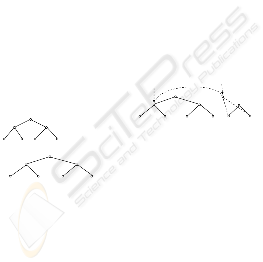
In Fig. 4, we show how T
1
is checked against <S
1
, ...,
S
l
>. In the figure, 1
(k)
stands for a sequence
containing k 1s, and then
)(
1
k
T represents the left-
most subtree of
)1(
1
−k
T
’s root. For instance,
)3(
1
T
(i.e., T
111
) is the left-most subtree of the root of
)2(
1
(i.e., TT
11
). When we check T
1
against <S
1
, ...,
S
l
>, we will look for an i such that |T
1
| ≥ |<S
1
, ...,
S
i
>| but |T
1
| < |<S
1
, ..., S
i+1
>|. Then, we will check
)2(
1
against <ST
1
, ..., S
i
>. When we do this, the same
method applies. We repeat this process until we
meet
)(
1
k
for some k such that |ST
1
| ≤ | | < |<S
)(
1
k
T
1
,
S
2
>|. In this case, we will check against S
)(
1
k
T
1
in a
top-down fashion as discussed above. If
includes S
)(
1
k
T
1
, we will try to check whether
21
)1( −k
T , the
direct right sibling subtree of
, includes <S
)(
1
k
T
2
, ...,
S
j
> for some j such that |<S
2
, ..., S
j
>| ≤ |
21
)1( −k
T
| <
|<S
2
, ..., S
j+1
>|. Otherwise, we will check whether
21
)1( −
includes <S
k
T
1
, ..., S
h
> for some h such that
|<S
1
, ..., S
h
>| ≤ |
21
)1( −k
T
| < |<S
1
, ..., S
h+1
>|. Obviously,
the whole computation is a top-down process with
the bottom-up checkings interleaved. Concretely,
the top-down and the bottom-up processes are mixed
as follows.
- Let T’ be a subtree of T. If there exists an i (> 1)
such that |<S
1
, ..., S
i
>| ≤ |T’| < |<S
1
, ..., S
i+1
>|, we
will check T’ against <S
1
, ..., S
i
> in a bottom-up
way. That is, we will first check whether the
subtrees of the root of T’ include <S
1
, ..., S
i
>.
- If |<S
1
>| ≤ |T’| < |<S
1
, S
2
>|, we will check T’
against S
1
top-down, by which we will first
compare the root of T’ and the root of S
1
.
Since the top-down and bottom-up processes are
mixed, we need to find a way to distinguish them.
Consider the recursive call to check
)2(
1
T
against
<S
1
, ..., S
i
> illustrated in Fig. 4. If the return value is
0, it shows that the subtrees of
)2(
1
T ’s root does not
contain any subtree in <S
1
, ..., S
i
>. However,
itself may includes S
)2(
1
T
1
. So we need to check
)2(
1
T
against S
1
once again. Now, we consider the
recursive call to check
)(
1
k
T
against <S
1
> illustrated
in Fig. 4. In this case, both
)(
1
k
T and <S
1
> are trees.
If the return value is 0, it shows that
)(
1
k
T itself does
not include S
1
. Then, a second checking as above is
not needed. To avoid such a second checking, we
mark the root of
when it is checked against the
root of S
)(
1
k
T
1
.
In terms of the above observation, we devise a
computation process as below. First of all, in the
case of label(r
1
) = label(r
2
), we will check whether
T
1
includes <S
1
, ..., S
l
>. The process returns an
integer i, indicating that T
1
includes <S
1
, ..., S
i
>. If i
> 0, then we will check whether T
2
includes
<S
i+1
, ..., S
l
> in a next step. If i = 0, it shows that no
subtrees of T
1
’s root includes any subtrees in
<S
1
, ..., S
l
>. In this case, we need to check whether
T
1
includes S
1
. It is because although no subtrees of
T
1
’s root includes any subtrees in <S
1
, ..., S
i
>, T
1
itself may include S
1
. If T
1
includes S
1
, i will be
changed to 1; otherwise, it remains 0. However, if
the root of T
1
does not match the root of S
1
, we know
that T
1
cannot include S
1
since in this case we will
have to check the subtrees of T
1
’s root against S
1
;
and we have already done that with the result i = 0.
We repeat this process until we find a k
j
such that
checking against
<S
1
, …, S
l
>
T
1
j
k
contains all the remaining subtrees of rT
2
, or find
that such a k
j
does not exist.
In the following algorithm tree-inclusion(T, S), T is
a tree and S is a tree or a forest. If S is a forest, a
virtual root for it is constructed, which matches any
label. Thus, we will actually check the subtrees of
T’s root against the subtrees in S, respectively. In
this way, a top-down process is switched over to a
bottom-up process. In addition, each node v in T is
associated with a mark, denoted mark(v). If v’s label
is checked against the label of a node S, its mark is
temporarily set to 1 to avoid possible redundant
checkings. But the mark may be dynamically
changed in the subsequent execution.
T
1
(2)
<S
1
, …, S
i
> (i ≤ l)
checking against
recursive call
<S
1
>
checking against
T
1
(k)
Figure 4: Illustration for calling top-down process
ICEIS 2005 - DATABASES AND INFORMATION SYSTEMS INTEGRATION
186

Function tree-inclusion(T, S)
Input: T - target tree; S - pattern tree.
Output: 1 if T includes S; 0 if T doesn’t include S.
begin
1. if |T| < |S| then {if S is a forest: <S
1
, ..., S
l
>
2. then S := <S
1
, ..., S
i
> for some i such that
|<S
1
, ..., S
i
>| ≤ |T| < |<S
1
, ..., S
i
+1>|
3. else return 0;}
4. let r
1
and r
2
be the roots of T and S, respectively;
5. (*If S is a forest, construct a virtual root r2 for it,
which matches any label.*)
6. let T
1
, ..., T
k
be the subtrees of r
1
;
7. let S
1
, ..., S
l
be the subtrees of r
2
;
8. if label(r
1
) = label(r
2
)
9. then {if r
1
is a leaf then {if r
2
is not a virtual root
then return 1 else return 0;}
10. if r
2
is not a virtual root then mark(r
1
) := 1;
11. temp := <S
1
, ..., S
l
>; S
0
:= φ;
12. i := 1; j := 0; x := 0; (*i is used to scan T
1
, ..., T
k
; and
j is used to scan S
1
, ..., S
l
.*)
13. while (i
≤ k ∧ temp ≠ φ) do
14. {x := tree-inclusion(T
i
, temp);
15. if x > 0 then temp := temp/<S
j
+1, ..., S
j
+x>;
16. else
{let v be the T
i
’s root; let u be the S
j
+1’s root;
17. if v and u have the same label and mark(v) = 0
18. then {x := tree-inclusion(T
i
, S
j
+1);
temp := temp/<S
j
+x>;}
(*In the case that j = 0 and x = 0, S
j
+x = S
0
= φ.*)
19. else mark(v) := 0}
(*mark(v) is used only once in this case. Afterwards,
it will be set to 0 for the subsequent computation.*)
20. i := i + 1; j := j + x;}
21. if temp ≠ φ then {if r
2
is a virtual root then
return j
22. else return 0;}
23. else {if r
2
is a virtual root then return l
24. else return 1;}}
25. else {for i = 1 to k do
26. { x := tree-inclusion(T
i
, S);
27. if x = number-of-trees(S) then return 1;}
(* number-of-trees(S) is the number of the trees in S. A
tree can be considered as a forest containg only that tree.*)
28. return 0;}
end
In Algorithm tree-inclusion(T, S), line 1 checks
whether |T| < |S|. If it is the case, the algorithm
returns 0 if S is a tree. If S is a forest, we will check
T against the first i subtrees such that |<S
1
, ..., S
i
>|
≤ |T| < |<S
1
, ..., S
i+1
>| (see line 2). In addition, when
we check T against a forest <S
1
, ..., S
l
>, a virtual root
for it is constructed, which matches any label. Thus,
we will actually check the subtrees of T’s root:
T
1
, ..., T
k
against S
1
, ..., and S
l
to see whether they
include <S
1
, ..., S
l
> (see line 5). This is performed in
a while-loop over T
i
’s. In each step, a
recursive call: tree-inclusion(T
i
, <
i
l
, ..., S
S
l
>) (i = 1,
..., j for some j) is carried out, which returns an
integer x, indicating that T
i
includes <
i
l
, ...,
1−+ xl
i
> (see line 14). If x = 0, i.e., the subtrees of
T
S
S
i
’s root do not include any subtree in
i
l
, ..., SS
l
, we
need to check whether T
i
include
i
l
since when we
check T
S
i
against
i
l
, ..., S
S
l
, what we have really
done is to check the subtrees of T
i
’s root, not T
i
itself
(see lines 16 - 19). If S is a tree, the algorithm return
1 if it is included; otherwise, 0 (see line 22 and 24).
Finally, we note that if the root of T does not match
the root of S, the algorithm tries to find the first T
i
that contains the whole S (see lines 25 - 28).
In addition, we should pay attention to how mark(v)
is used (see lines 10, 17, and 19). Each time when v
is checked against a node (not a virtual node) in S,
mark(v) is set to 1. It is used to avoid the call tree-
inclusion(T[v], S
j
+1) after tree-inclusion(T[v], <S
j+1
,
..., S
l
>) returns back if |S
j+1
| ≤ |T[v]| < |<S
j+1
, S
j+2
>|
(see line 17), where T[v] represents a subtree (in T)
rooted at v. It is because in this case tree-
inclusion(T[v], S
j+1
) must have been invoked during
the execution of tree-inclusion(T[v], <S
j+1
, ..., S
l
>)
and v has been definitely checked against S
j
+1’s root
in this process, which is recorded by setting mark(v)
to 1 and used to avoid a second checking. However,
it is used only in this case. After that, it should be set
to 0 again for the rest part of the computation. This
arrangement is correct because during the execution
of tree-inclusion(T[v], <S
j+1
, ..., S
l
>), if |S
j+1
| ≤ |T[v]|
< |<S
j+1
, S
j+2
>|, v itself will be checked against S
j+1
’s
root. If |T[v]| ≥ |<S
j+1
, ..., S
j+i
>| for some i > 1, we
will check the subtrees of v against <S
j+1
, ..., S
j+i
>
and v is not really checked. In addition, in the rest
part of the execution of tree-inclusion(T[v], <S
j+1
, ...,
S
l
>), v is not checked. So, upon the return of tree-
inclusion(T[v], <S
j+1
, ..., S
l
>), we check the value of
mark(v) to see whether tree-inclusion(T[v], S
j+1
) has
been invoked. Obviously, after this checking,
mark(v) should be set to 0 again for the subsequent
computation.
Finally, we can show that the time complexity of the
algorithm is bounded by O(|T|⋅height(S)). It is
because although a node in T may be checked more
than once, it is checked against different nodes in S,
and all those nodes in S are on a same path. It is also
easy to see that the algorithm needs no extra space.
In the following, we apply the algorithm to the trees
shown in Fig. 5 and trace the computation step-by
step for a better understanding.
Example 2. Consider two ordered, labeled trees T
and S shown in Fig. 5, where each node in T is
identified with t
i
, such as t
0
, t
1
, t
11
, and so on; and
ON THE TREE INCLUSION AND QUERY EVALUATION IN DOCUMENT DATABASES
187

each node in S is identified with s
j
. In addition, each
subtree rooted at t
i
(s
j
) is represented by T
i
(S
j
).
In the following step-by-step trace, i
k
is used as an
index variable for scanning the subtrees of T
k
’s root;
j
k
is used to scan the corresponding subtrees in S;
and x
k
is used as a temporary variable.
4 INTEGRATION OF
SIGNATURES INTO TREE
INCLUSION
An advantage of the top-down strategy is that we
can integrate the signature technique into the tree
inclusion to speed up the computation. We assign
each node v in T a bit string s
v
, called a signature,
and each node u in S a bit string s
u
in such a way that
if s
u
matches s
v
then the subtree T
v
rooted at v may
includes the subtree S
u
rooted at u. Otherwise, T
v
definitely does not contain S
u
and the corresponding
tree inclusion checkings can be cut off. Here, by
“matching”, we mean for each bit set to 1 in s
v
, the
corresponding bit in s
u
is also set to 1 while for a bit
set to 0 in s
v
, the corresponding bit in s
u
can be 0 or
1.
t
1
t
2
d
c
e
c
b
e
t
21
t
11
t
12
t
22
d
c
a
s
0
s
1
S:
s
2
Figure 5: Two trees
Step-by-step trace: Explanation:
tree-inclusion(T, S) Call tree-inclusion(T, S)
label(t
0
) = label(s
0
) Check t
0
against s
0
.
i
0
:= 1; j
0
:= 0; x
0
:= 0 i
0
is for scanning the subtrees of t
0
; j
0
is used to record how many
subtrees of s
0
is included; x
0
is a temporary variable.
tree-inclusion(T
1
, <S
1
, S
2
>) recursive call tree-inclusion(T
1
, <S
1
, S
2
>).
label(t
1
) = label(virtual-root) Check t
1
against a virtual root. It always succeeds.
i
1
:= 1; j
1
:= 0; x
1
:= 0 i
1
is for scanning the subtrees of t
1
; j
1
is used to record how many
subtrees of s
0
is included; x
1
is a temporary variable.
tree-inclusion(T
11
, <S
1
, S
2
>) recursive call tree-inclusion(T
11
, <S
1
, S
2
>).
|T
11
| < |<S
1
, S
2
>| compare the sizes of T
11
and <S
1
, S
2
>.
remove S
2
from <S
1
, S
2
> since <S
1
, S
2
> is larger than T
11
, remove S
2
from <S
1
, S
2
>.
label(t
11
) = label(s
1
) Check t
11
against s
1
. Mark t
11
.
return 1 it returns 1, indicating that T
11
includes S
1
.
x
1
= 1; j
1
= 1; i
1
= 2 i
1
is increased by 1; x
1
is equal to 1 and then j
1
is increased by 1.
tree-inclusion(T
12
, S
2
) recursive call tree-inclusion(T
12
, S
2
).
label(t
12
) ≠ label(s
2
) Check t
12
against s
2
. Mark t
12
.
return 0 it returns 0, indicating that T
12
does not include S
2
. The mark of t
12
will prevent
the second checking of t
12
against S
2
.
x
1
= 0; j
1
= 1; i
1
= 3 i
1
is increased by 1; x
1
is equal to 0 and then j
1
is not increased.
return 1 it returns 1, indicating that T
1
includes S
1
of <S
1
, S
2
>.
x
0
= 1; j
0
= 1; i
0
= 2 i
0
is increased by 1; x
0
is equal to 1 and then j
0
is increased by 1.
tree-inclusion(T
2
, S
2
) recursive call tree-inclusion(T
2
, S
2
).
label(t
2
) ≠ label(s
2
) Check t
2
against s
2
. Since they do not match, all the subtrees of t
2
will be
checked one by one.
i
2
:= 1; j
2
:= 0; x
2
:= 0 i
12
is for scanning the subtrees of t
2
; j
1
is used to record how many
subtrees of s
0
is included; x
2
is a temporary variable.
tree-inclusion(T
21
, S
2
) recursive call tree-inclusion(T
21
, S
2
).
label(t
21
) ≠ label(s
2
) Check t
21
against s
2
. Mark t
21
.
return 0 it returns 0, indicating that T
21
does not include S
2
. The mark of t
21
will prevent
the second checking of t
21
against S
2
.
x
2
= 0; j
2
= 0; i
2
= 2 i
2
is increased by 1; x
2
is equal to 0 and then j
2
is not increased.
tree-inclusion(T
22
, S
2
) recursive call tree-inclusion(T
22
, S
2
).
label(t
22
) = label(s
2
) Check t
22
against s
2
. Mark t
22
.
return 1 it returns 1, indicating that T
22
includes S
2
.
x
2
= 1; j
2
= 1; i
2
= 3 i
2
is increased by 1; x
2
is equal to 1 and then j
2
is increased by 1.
return 1 it returns 1, indicating that T
2
includes S
2
of <S
1
, S
2
>.
x
0
= 1; j
0
= 2; i
0
= 3 i
0
is increased by 1; x
0
is equal to 1 and then j
0
is not increased by 1.
return 2 since j
0
= 2, tree-inclusion(T
2
, S
2
) returns 2.
return 1 it returns 1, indicating that T includes S.
ICEIS 2005 - DATABASES AND INFORMATION SYSTEMS INTEGRATION
188

To do this, we firs assign each label a signature by
using a hash function as doen in (C. Faloutsos ,
1992). Then, the signature for each node in a labeled
tree can be done as follows:
Let v be a node in a tree T. If v is a leaf node, its
signature s
v
is equal to the signature assigned to its
label.
Otherwise, let v
1
, ..., v
n
be its children, then s
v
= s ∨
1
v
∨ ... ∨
n
v
, where s represents the signature for
the label associated with v, and
1
v
, ... , and are
the signatures of v
s s
s
n
v
s
1
, ..., v
n
, respectively.
Example 3. Consider the tree shown in Fig. 6(a). If
the signatures assigned to the labels are those shown
in Fig. 6(b). Each node in the tree will have a
signature as shown in Fig. 6(c).
Given two ordered, labeled trees T and S, we assign
the signatures to their nodes in the same way.
During the checking whether T includes S, we can
use signatures to cut off some subtrees of T, which
cannot contain S. For this purpose, we change the
algorithm tree-inclusion( ) by introducing the
signature checkings into it. The following algorithm
is almost the same as the algorithm tree-inclusion( );
but each time when we check whether a subtree of T
includes a subtree of S, the corresponding signatures
will be first checked. Of course, before the execution
of the algorithm, the node signatures have to be
established for both T and S.
Algorithm signature-tree-inclusion(T, S)
Input: T, S
Output: 1, if T includes S; otherwise, 0.
begin
1. if |T| < |S| then {if S is a forest: <S
1
, ..., S
l
>
2. then S := <S
1
, ..., S
i
> for some i such that
|<S
1
, ..., S
i
>| ≤ |T| < |<S
1
, ..., S
i
+1>|
3. else return 0;}
4. let r
1
and r
2
be the roots of T and S, respectively;
5. (*If S
is a forest, construct a virtual root for it, which
matches any label.*)
6. let t
and s be the signatures of T and S , respectively;
7. if s does not match t then returns 0;
8. let T
1
, ..., T
k
be the subtrees of r
1
;
9. let S
1
, ..., S
l
be the subtrees of r
2
;
(*the rest part of the algorithm is exactly the same as lines
8 – 28 in Algorithm tree-inclusion( ).*)
end
We pay attention to line 5. If S is a forest, a virtual
root for S will be constructed and it does not have a
signature. However, its signature can be easily
established by superimposing the signatures of all
the subtrees in S. Then, in lines 6 and 7, we check
the corresponding signatures to remove the
checkings for impossible tree inclusion.
Example 4. Consider the tree T and S shown in Fig.
5 again. To check whether T includes S, we will
assign signatures to the labels and the nodes in T and
S in the same way as shown in Fig. 7. Assume that
the assignment of the signatures to the labels is
shown in Fig. 6(b). Then, the checking of the forest
containing s
1
and s
2
(in S) against the tree rooted at t
1
(in T) can be avoided. It is because the signature for
the virtual node of the forest (equal to 0011 1101)
does not match the signature for t
1
(equal to 1111
1000).
5 CONCLUSION
In this paper, a new strategy for evaluating path-
oriented queries are discussed. The main idea of the
query evaluation is a new algorithm for checking the
inclusion of a query tree S in a document tree T, by
which a top-down process is interleaved with a
bottom-up computation. The algorithm has the time
complexity comparable to the best bottom-up
method, but needs no extra space. In addition, it is
more suitable for a database environment and can be
combined with the signature technique to get rid of
useless checkings for subtree inclusion. Obviously,
this cannot be achieved using any bottom-up
strategy.
REFERENCES
W. Chen. More efficient algorithm for ordered tree
inclusion. Journal of Algorithms, 26:370-385, 1998.
R. Cole, R. Hariharan, P. Indyk. Tree pattern matching
and subset matching in deterministic O(n log^3 m)
e
1111 1000
t
22
t
12
t
0
t
1
t
2
d c
f
b
e
a
t
21
t
11
1111 1101
1100 0000
1010 1000
1111 1101
0001 0101 0010 1000
Figure 7: Cutting off subtrees using
i
S:
s
0
s
1
d
c
a
s
2
0001 0101
0010 1000
0011 1101
This subtree
will
bld
virtual node
T:
not match
a: 0101 0000
b: 0011 1000
c: 0001 0101
d: 0010 1000
e: 1010 1000
f
: 1100 0000
t
1
t
2
d
c
e
f
b
e
a
t
21
t
11
t
0
T:
t
12
t
22
(a)
(b)
t
0
1111 1000
t
22
t
12
t
1
t
2
d c
e
f
b
e
a
t
21
t
11
1111 1101
1100 0000
1010 1000
1111 1101
0001 0101 0010 1000
(c)
Figure 6: Node signatures
ON THE TREE INCLUSION AND QUERY EVALUATION IN DOCUMENT DATABASES
189

time. Proceedings of the Tenth Annual ACM-SIAM
Symposium on Discrete Algorithms (SODA), 1999,
245-254.
A. Deutsch, M. Fernadez, D. Florescu, A Levy, and D.
Suciu, XML-QL: A Query Language for XML,
Technical report, World Wide Web Consortium, 1989,
http://www.w3.org/TR/ Note-xml-ql.
C. Faloutsos, “Signature Files,” in: Information Retrieval:
Data Structures & Algorithms, edited by W.B. Frakes
and R. Baeza-Yates, Prentice Hall, New Jersey, 1992,
pp. 44-65.
GMD. Gmd-ipsi xql.engine.
http://xml.dramstadt.gmd.de/xql/ index.html, August
1999.
C. Zhang, J. Naughton, D. DeWitt, Q. Luo and G.
Lohman, “On Supporting Containment Queries in
Relational Database Management Systems, in Proc. of
ACM SIGMOD Intl. Conf. on Management of Data,
California, USA, 2001.
INRIA. Minixyleme project.
http://www.rocq.inria.fr/~aguilera/xoql/minixyleme/re
adme.html.
Pekka Kilpelainen and Heikki Mannila. Ordered and
unordered tree inclusion. SIAM Journal of Computing,
24:340-356, 1995.
H. Mannila and K.-J. Raiha, On Query Languages for the
p-string data model, in “Information Modelling and
Knowledge Bases” (H. Kangassalo, S. Ohsuga, and H.
Jaakola, Eds.), pp. 469-482, IOS Press, Amsterdam,
1990.
Thorsten Richter. A new algorithm for the ordered tree
inclusion problem. In Proceedings of the 8th Annual
Symposium on Combinatorial Pattern Matching
(CPM), in Lecture Notes of Computer Science (LNCS),
volume 1264, pages 150-166. Springer, 1997.
J. Robie, J. Lapp, and D. Schach, XML Query Language
(XQL), 1998. http://www.w3.org/TandS/QL/QL98/pp/
xql.html.
J. Shanmugasundaram, K. Tufte, G. He, C. Zhang, D.
DeWitt, J. Naughton, “Relational Databases for
Querying XML Documents: Limitations and
oppotunities,” Proc. VLDB, Edinburgh, Scotland,
1999.
World Wide Web Consortium, Extensible Markup
Language (XML) 1.0.
http//www.w3.org/TR/1998/REC-xml/19980210,
Febuary 1998.
World Wide Web Consortium, Extensible Style Language
(XML) Working Draft, Dec. 1998.
http//www.w3.org/TR/ 1998/WD-xsl-19981216.
ICEIS 2005 - DATABASES AND INFORMATION SYSTEMS INTEGRATION
190