EARLY PERFORMANCE ANALYSIS IN THE DESIGN OF

SPATIAL DATABASES

Vincenzo Del Fatto, Massimiliano Giordano, Giuseppe Polese

Monica Sebillo and Genoveffa Tortora

Dipartimento di Matematica e Informatica, Università degli Studi di Salerno

Via Ponte don Melillo Fisciano (SA), Italy

Keywords: Conceptual Database Design, Spatial Databases, GIS.

Abstract: The construction of spatial databases often requires considerable computing and storage resources, due to

the inherent complexity of spatial data and their manipulation. Thus, it would be desirable to devise

methods enabling a designer to estimate performances of a spatial database since from its early design

stages. We present a method for estimating both the size of data and the cost of operations based on the

conceptual schema of the spatial database. We also show the application of the method to the design of a

spatial database concerning botanic data.

1 INTRODUCTION

Many techniques for designing spatial databases

have been devised by extending those used in the

design of traditional databases. In particular,

important extensions have regarded the conceptual

data models, which have interested both the Entity-

Relationship (Calkins, 1996; Chen, 1976), and the

Object-Oriented models (Price et al., 2000;

Rumbaugh et al., 1998). Traditional database design

techniques also provide means to produce an early

estimation of the database size and the access

performances, based on the conceptual database

schema (Atzeni et al., 1999; Elmasri and Navathe,

2004). So far, no similar techniques have been

proposed for the design of spatial databases, despite

in this context it is much more critical the early

estimation of both size and performances, due to the

complexity of geographic data. A late evaluation of

these aspects entails high design cost to review early

design decisions.

In this paper we propose a technique for

estimating size and performances of a spatial

database based on its conceptual schema. The

technique has been developed on the extended ER

model by Calkins (1996), but its principles can be

easily applied to other models. Basically, the

approach uses the constructs of the conceptual

schema to estimate disk occupancy, and access

performances. We have extended existing estimation

models for alphanumeric databases to add

parameters capable of expressing basic

characteristics of different spatial data types, and

that are measurable during the conceptual design

phase.

In order to opportunely tune the parameters of

our model we have performed massive experiments

to observe access performance trends when varying

the size and typology of spatial data. Our goal has

been to derive a single unit of measurement to

express estimated access performances for the

different types of data stored in a spatial database.

The paper is organized as follows. Section 2

provides a brief overview of the spatial database

design process. In Section 3 we present our

estimation method. Section 4 describes the

application of our method to a botanic database

example. Finally, Section 5 provides discussion and

final remarks.

2 THE SPATIAL DATABASE

DESIGN PROCESS

The process for the design of a spatial database

described in the literature follows similar guidelines

used for the design of traditional databases. In

particular, after requirements analysis, there are

often the conceptual, and the logical design phases.

The goal of the conceptual phase is to analyse

data requirements and to model them according to a

172

Del Fatto V., Giordano M., Polese G., Sebillo M. and Tortora G. (2007).

EARLY PERFORMANCE ANALYSIS IN THE DESIGN OF SPATIAL DATABASES.

In Proceedings of the Second International Conference on Software and Data Technologies - Volume ISDM/WsEHST/DC, pages 172-177

DOI: 10.5220/0001343001720177

 SciTePress

conceptual spatial data model. In order to overcome

limitations of traditional ER and Object-Oriented

models, which do not provide means to describe

spatial data in an abstract way, conceptual data

models have been extended to provide means to

abstractly represent characteristics of spatial data

(Hadzilacos and Tryfona, 1997; Shekhar et al.,

1997; Tryfona and Jensen, 1999). In the rest of the

paper we will use an extension of the ER model,

namely the Calkins model (Calkins, 1996), in order

to present our method and to illustrate examples, due

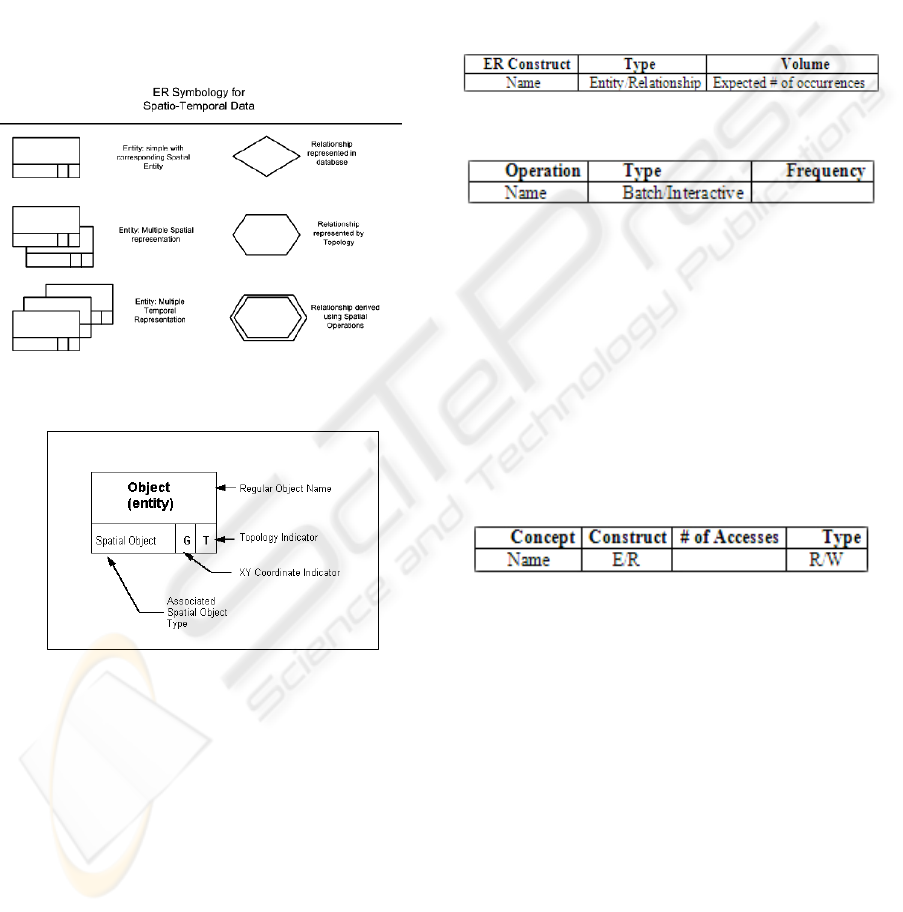
to its simplicity and intuitiveness. Figure 1 and 2

show the symbols of this model.

Figure 1: Calkins conceptual data model notation.

Figure 2: The Entity Symbol for Spatial Objects.

Once the conceptual schema has been produced, it is

used as input to the logical design phase.

The goal of the logical design phase is to

translate the input conceptual schema into a logical

schema abiding by the formalism of a given logical

spatial data model. Before facing the translation

task, a restructuring of the conceptual schema is

usually performed. In the literature on traditional

databases there are slight variants for this phase. In

what follows we review one of such methods,

namely, the one introduced by Atzeni et al. (1999),

where the workload represents an estimation of

database performances in terms of expected disk

space occupancy, and accesses by main operations.

The information about the workload is

represented through three types of tables (Atzeni et

al., 1999): Volumes Table, Operations Table, and

Accesses Table, shown in Tables 1-4.

The designer can use the information provided in

these tables to formally compare alternative schema

restructuring choices. In particular, s/he can evaluate

the impact that each choice would produce on the

workload in terms of both space occupancy and

operation performances.

Table 1: Volumes Table.

Table 2: Operations Table.

Based on the rule by which 80% of the workload for

a database system is generated by the 20% of the

most frequent operations (Atzeni et al., 1999), in this

phase the designer aims to detect this last set of

operations. They will be the ones s/he inserts in the

operations table, producing for each of them an

access table describing the ER constructs to be

visited when executing it. In table 3 the symbols

R/W indicate access type, R for reading, and W for

writing.

Table 3: Accesses Table.

After the restructuring phase has been

completed, the restructured schema is translated into

a logical schema by using mapping rules that are

specific of the chosen logical data model. No such

estimation methods exist for the spatial database

domain. In the next section we discuss our proposal.

3 PERFORMANCE

EVALUATION ON SPATIAL

CONCEPTUAL SCHEMES

As opposed to analogous methods for traditional

databases, the early estimation of performances for

spatial databases is a considerably more complex

task, due to the inherent complexity of the data they

manage. On the other hand, the availability of a

EARLY PERFORMANCE ANALYSIS IN THE DESIGN OF SPATIAL DATABASES

173

proper estimation method would produce increased

benefits. In fact, while for traditional databases disk

occupancy is not a major concern, also due to the

reduced cost of storage devices, different design

choices for spatial databases can yield huge

differences in terms of disk occupancy and response

time for spatial data processing.

In order to produce an estimation of disk

occupancy of a spatial database it is necessary to

take into account the different data formats that can

be associated with the spatial component of a

geographic data, namely raster, and vector. When

trying to express the volume of data featuring a

spatial dataset, it is necessary to take into account

the dual nature of a spatial data, i.e. it is made of two

components, namely descriptive and geometric

components. To this end, in addition to traditional

volume tables used in alphanumeric databases, we

introduce two new volume tables, one for vector and

one for raster spatial data. The structure of the vector

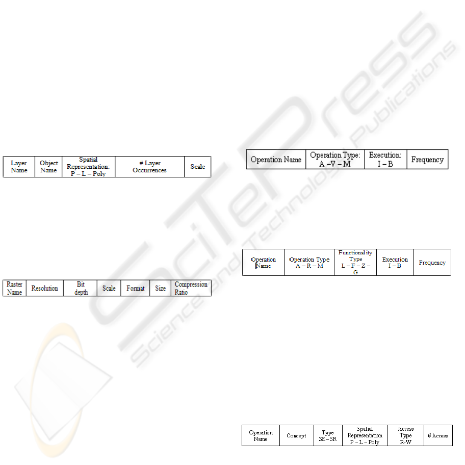
volumes table is defined as follows:

Table 4: Vector Volume Table.

It contains the layer name, the object name, the

spatial representation (Point, Line, Polygon), the

number of layer occurrences, and the Scale.

The structure of the raster volumes table is

defined as follows:

Table 5: Raster Volume Table.

It contains the raster name, its resolution (measured

in ppi - pixel per inches), the bit depth (the number

of bits used for each pixel), the scale, the file format,

the file size (measured in MB), and the compression

ratio. The latter applies to compressed raster data,

for which neither resolution nor bit depth apply.

As for data processing operations, spatial

databases should enable users to accomplish

intensive query and analysis sessions on very large

data, to be conducted either on separate components,

or simultaneously on spatial and descriptive

components. Both these types of operations are

divided into two categories: vector and raster.

Vector (resp. raster) operations are classified as

follows:

 alphanumeric: they work either on

alphanumeric data or on the descriptive

component of spatial data;

 vector (resp. raster): they work on the vector

(resp. raster) component of spatial data;

 mixed: they work on both vector (resp. raster)

and descriptive components of spatial data.

Moreover, raster operations may be also

classified on the basis of the functionality type they

invoke:

 zonal: they perform a cross-tabulation using

zones of two input themes;

 local: they calculate output values based on

values from multiple grids at same location;

 focal: they calculate statistics on cells found

within a neighbourhood;

 global: they calculate output values based on all

values of the input theme.

To produce an estimation of the computation time

for spatial data processing operations, we introduce

two additional operation tables, namely vector and

raster operation tables, and two additional access

tables, namely vector access table, and raster access

table. These are defined as follows:

Table 6: Vector Operations Table.

It contains operation name, operation type

(Alphanumeric, Vector, Mixed), execution type

(Interactive, Batch), and operation frequency.

Table 7: Raster Operations Table.

It contains operation name, operation type

(Alphanumeric, Raster, Mixed), functional type

(Local, Focal, Zonal, Global), execution type

(Interactive, Batch), and operation frequency.

For each operation listed in one of the operation

tables there is an access table showing entities and

relationships it needs to access during its execution.

The structure of the vector access table is defined as

follows:

Table 8: Vector Access Table.

It contains the operation name, the schema construct,

the type (spatial entity, spatial relationship), the

access type (Read, Write), the spatial representation

(Point, Line, Polygon), and the number of accesses.

Finally, the structure of the raster access table is

described as follows:

ICSOFT 2007 - International Conference on Software and Data Technologies

174

Table 9: Raster Access Table.

It contains the operation name, the schema construct,

the number of accesses, and the access type (Read,

Write).

Although these tables provide an overview of the

database performances, we can derive a unique unit

of measurement to express the cost of operations in

terms of accesses to the database, independently

from the type of data on which they are performed.

To do this, we have performed massive experiments

on real applications involving large heterogeneous

spatial datasets. The testing environment is based on

PostgreSQL 8.1 with GIS extension POSTGIS, Dual

Intel Xeon system with 2G of ram and Windows XP

pro.

We have executed several operations involving

different spatial data types, and have measured

several performance indicators, such as execution

time, RAM usage, and volume of data exchanged

with mass storage devices. The latter is the indicator

on which we have based the parameters for our

estimation model, since it guarantees invariance

with respect to the hardware used, and it is not

affected by the noise introduced by the measurement

software itself.

Traditional estimation methods for alphanumeric

databases only consider the different complexity of

read with respect to write accesses, since they are all

alphanumeric. In our case, other than differentiating

between read and write accesses, we have focused

on the following main types of data: alphanumeric,

points, lines, and polygons. The notation used to

express the different types of accesses and the types

of data on which they are performed follows:

RAN = Access cost to read an alphanumeric data

WAN = Access cost to write an alphanumeric data

RPT = Access cost to read a point

WPT = Access cost to write a point

RLN = Access cost to read a line

RPL = Access cost to read a polygon

WPL = Access cost to write a polygon

RRS = Access cost to read a raster image

WRS = Access cost to write a raster image

We observed that access performances of the

spatial data point are similar to those of average

size alphanumeric data. Moreover, we observed

that access performances of lines and polygons

grow linearly with the number of vertices. We also

noticed that RLN entails higher costs than RPL

due to the different storage methods that the Open

Geospatial Consortium defines for these two data

types (OGC, 2007). Since we do not have info on

the expected number of vertices for these types of

data during the conceptual design phase, we

needed to estimate the cost of access operations on

them independently from this parameter. To this

end, we observed that varying the number of

vertices from few up to 1000, for both types of

geometries, entailed a volume of data exchanged

with mass storage devices varying from 0,5 to 2

MB. Thus, since the number of vertices of most

real geometries falls in this range, we can assume

that the average number of MB exchanged is O(1).

In conclusion, we have derived the following

relationships:

RPT ≅ RAN; WPT ≅ WAN ≅ 7*RPT;

RPL ≅ 70*RPT; RLN ≅140*RPT;

WLN ≅ WPL ≅ 350*WPT

We have assigned the value 1 to RAN and RPT,

yielding the following relationships:

RPT ≅ RAN ≅ 1; WPT ≅ WAN ≅ 7

RPL ≅ 70; RLN ≅ 140;

WLN ≅ WPL ≅ 350

As for raster images, finding a proper

estimation at conceptual level is more complex a

task, because we do not know yet parameters like

resolution, compression, and bit depth, which

would be useful to estimate the bytes to be

exchanged with mass storage to manipulate them.

Moreover, it is more difficult to characterize the

types of operations and their access costs before

lower level design stages. Nevertheless, in our

experiments we have noticed that for images with

resolution ranging from 48.000 pixels to 2 Mega

pixels, bit rate from 16 to 32 bits, stored through

well known compressed formats they occupy from

0,5 to 10 MB of disk space. Thus, the designer can

opportunely tune the estimated cost of operations

on raster images depending on the knowledge s/he

has about the images to handle at this stage of the

design process. From what said above, for images

without a particularly big size we can estimate an

average number of bytes exchanged which is twice

than that of vector images.

4 CASE STUDY

The ER schema shown in figure 3 represents the

conceptual schema for a portion of a spatial database

EARLY PERFORMANCE ANALYSIS IN THE DESIGN OF SPATIAL DATABASES

175

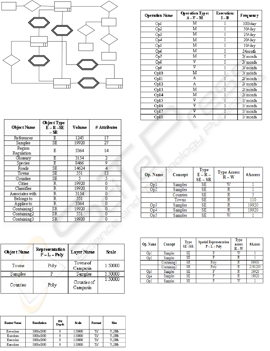
of botanic data. Part of workload for this schema is

summarized in Tables 10-12.

Cities

(0,N) (1,1)

References

Classifies

Species

Samples

Point

Associates with

Glossary

Applies to

Region

Regulation

Containing4

Containing2

Containing3

Containing1

Containing5

Belongs to

Towns

Polygon

Counties

Polygon

Roads

Line

(1,1)

(0,N)

(1,1)

(0,N)

(1,N)

(0,N)

(1,1)

(0,N)

(1,1)

(0,N)

(1,1)

(1,N)

(0,1)

Cities

(0,N) (1,1)

References

Classifies

Species

Samples

Point

SamplesSamples

Point

Associates with

Glossary

Applies to

Region

Regulation

Containing4

Containing2

Containing3

Containing1

Containing5

Belongs to

Towns

Polygon

TownsTowns

Polygon

Counties

Polygon

CountiesCounties

Polygon

Roads

Line

RoadsRoads

Line

(1,1)

(0,N)

(1,1)

(0,N)

(1,N)

(0,N)

(1,1)

(0,N)

(1,1)

(0,N)

(1,1)

(1,N)

(0,1)

Figure 3: ER schema of the Botanic Spatial Database.

Table 10: Alphanumeric Volume Table.

Table 11: Vector Volume Table.

Table 12: Raster Volume Table.

Regarding operations, we had 28 operations. In

Table 13 we report the 18 most frequent of them.

Table 13: Alphanumeric and Vector Operations Table.

Among these, we have developed Access Tables for

the first five most frequent and meaningful

operations (see Tables 14 and 15).

Table 14: Non Spatial Access Table.

Table 15: Vector Access Table.

In these tables we have distinguished read and

write operations on alphanumeric and vector data. In

the following we show redundancy analysis and

access performances for op4.

For each botanic sample, given an area

surrounding it (named buffer zone), this operation

requires the computation of the number of botanic

samples observed in the area. Since we store the

coordinates of each sample, and the ray of the

ICSOFT 2007 - International Conference on Software and Data Technologies

176

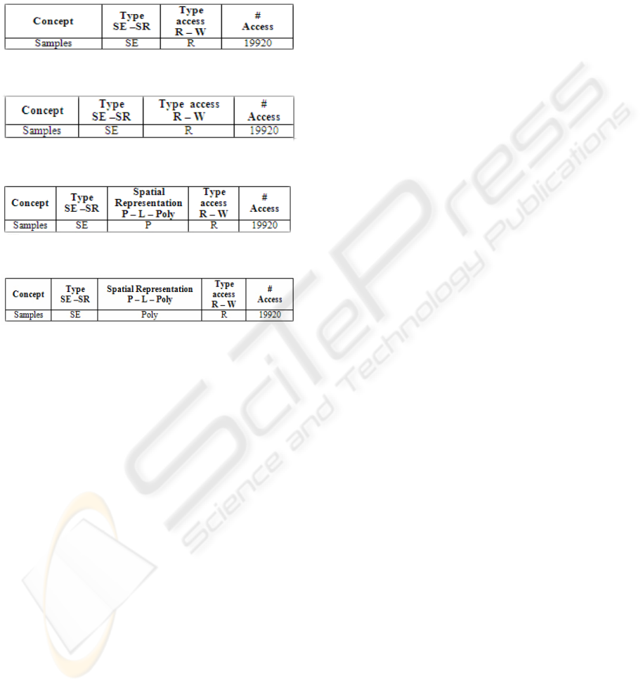
associated buffer zone, this last data becomes

redundant. To this end, the choice whether to keep

or remove such attribute is made based on the access

tables (Tables 16, 17, 18 and 19) developed for both

design alternatives.

Table 16: Alphanumeric Accesses without redundancy.

Table 17: Alphanumeric Accesses with redundancy.

Table 18: Vector Accesses without redundancy.

Table 19: Vector Accesses with redundancy.

By applying our method we obtain a total cost of

28.286.400 with redundancy, and 796.800 without

redundancy. Thus, we would conclude that is not

convenient to store the buffer zone, since we not

only save on the cost of accesses, but we also save

9.561.600 bytes of disk space. To experimentally

verify this, we have implemented both design

alternatives, observing that the time required by op4

with the redundant data is about 46 seconds,

whereas without it is about 556 ms. Obviously, the

last two parameters heavily depend on hardware

characteristics.

5 DISCUSSION

We have described a method to analyse the

performances of a spatial database since from early

stages of the design process. We have tuned its

parameters after several experiences in designing

and implementing spatial databases and their

surrounding GIS applications for real world

problems. We have presented concepts through a

case study concerning the design of a spatial

database containing botanic data.

The proposed method can potentially help the

designer in evaluating the quality of the design

artefacts based upon an estimation of

performances they can yield. This can also help

him/her to prevent the construction of inefficient

databases, which would be too expensive to revise

after their implementation is completed.

In the future we would like to develop finer

estimation methods, traceable from the one

presented here, to be used in later phases of the

design process, when more parameters on spatial

data and their manipulation functions are known.

We would also like to extend our approach to

accomplish early performance analysis of spatial

databases used in real time systems.

REFERENCES

Atzeni, Ceri, Paraboschi, Torlone, 1999. Basi di dati,

McGraw-Hill.

Calkins, H., W., 1996. Entity Relationship Modeling of

Spatial Data for Geographic Information Systems. In

International Journal of Geographical Information

Systems.

Chen, P., P., 1976. The entity-relationship model - toward

a unified view of data. In ACM Transactions on

Database Systems.

Elmasri, R., Navathe, S., B., 2004. Fundamentals of

Database Systems, Addison-Wesley.

Hadzilacos, T., Tryfona, N., 1997. An Extended Entity-

Relationship Model for Geographic Applications. In

SIGMOD Record.

OGC, Open Geospatial Consortium specification

compliant prod. list. Retrieved March 8, 2007 from

www.opengeospatial.org/resource/products/compliant.

Price, R., Tryfona, N., Jensen, C., 2000. Extended

Spatiotemporal UML: Motivations, Requirements, and

Constructs. In Journal of Database Management.

Special Issue on UML.

Rumbaugh, J., Jacobson, I., Booch, G., 1998. The Unified

Modeling Language Reference Manual, Addison-

Wesley Object Technology Series.

Shekhar, S., Coyle, M., Goyal, B., Liu, D., Sarkar S.,

1997. Data models in geographic information systems.

In Communications of the ACM.

Tryfona, N., Jensen, C., 1999. Conceptual data modelling

for spatiotemporal applications. In Geoinformatica.

EARLY PERFORMANCE ANALYSIS IN THE DESIGN OF SPATIAL DATABASES

177