SMART DIFFERENTIAL PRESSURE SENSOR

Michal Pavlik, Jiri Haze, Radimir Vrba and Miroslav Sveda

Brno University of Technology, Udolni 53, CZ-60200 Brno, Czech Republic

Keywords: Pressure measurement, ultra-low power application, current loop, microcontroller overclocking, non-linear

interpolation.

Abstract: This paper presents design and assembly of mixed electronic circuitry for measured signal processing of the

capacitive difference pressure sensor, as well as analysis of the obtained results. The smart pressure sensor

provides values of measured pressure via 4 - 20 mA current loop output. The loop current is also used for

sensor circuitry supplying. This means that current consumption of the whole sensor electronics should be

less than 3.5 mA even in extended industrial temperature range from –40 to +125 °C.

1 INTRODUCTION

There are needs in some industrial branches to

measure difference between two pressures. The

differential measurement system is frequently used

for pressure measurements because of its good

temperature and time stability. The internal

schematic diagram of the differential pressure sensor

can be analyzed is a pair of capacitors sensing to

differential pressure actual values. These capacities

can be up to tens of picofarads. There is no direct

measuring of capacities, but capacities of measured

capacitors are converted to actual output frequency

of a pair of frequency oscillators controlled by

measured capacitors. The most important issue is the

precision of measurement. Total accuracy is required

to be better than that equivalent to 16 binary bits

resolution. Therefore frequency of 255 periods of

the output signal is averaged. The aim of this paper

is the description of the low-power and high-

precision measuring system design.

2 ELECTRONICS TOPOLOGY

The proposed electronic circuitry of the pressure

sensor can be split into three modular parts. Signal

processing of the differential pressure sensor is

realized by a pair of oscillators whose output

frequencies reflect the value of the measured

pressure. Consequently, galvanically separated part

including microcontroller converts the output

frequency values of the oscillators to digital code

values. Besides, embedded microcontroller

calculates non-linear correction of the measured

values and temperature calibration at the same time.

The output quantity of this part of electronic

circuitry is a digital calibrated value of pressure.

According to the desired extended temperature range

from -40 to + 125 °C of the proposed sensor, the

outputs of the oscillators are carried by signal

transformers.

Figure 1: Block diagram of system topology.

memory

oscillators

temperature

sensor

galvanic separation

microcontroller

DC-DC converter

HART protocol modulator

244

Pavlik M., Haze J., Vrba R. and Sveda M. (2007).

SMART DIFFERENTIAL PRESSURE SENSOR.

In Proceedings of the Fourth International Conference on Informatics in Control, Automation and Robotics, pages 244-248

DOI: 10.5220/0001632302440248

 SciTePress

The microcontroller controls galvanically separated

DC-DC changer that supplies oscillators, too. The

block diagram of the electronic circuitry topology is

shown in Fig. 1. A microcontroller is included in the

third part of electronics. The microcontroller is

mainly used for HART modulation of the loop

current communication. The second function of the

microcontroller is active regulation of the actual

current in the current loop by means of sensor

consumption supplying current control.

Interconnection between the second and third stage

of electronics is provided by the SPI bus. These two

parts are galvanically connected.

2.1 Oscillators

Even if oscillators are based on the two basic 555

circuits, there are a few circuitry modifications. Only

one of oscillators is running during actual running

phase of the measurement process. It results in

decreasing power consumption to nearly 65% of the

original one. The ultra low power and fast

comparators MAX939 are used. The crucial

parameters of the comparators are slew rate and

transfer time delay. The application of these

comparators represents the best solution in terms of

power consumption and speed ratio. The precision

of the measurement mainly depends on the reaction

time of the comparators or possibly on the spread of

the overshoot from the reference voltage. The

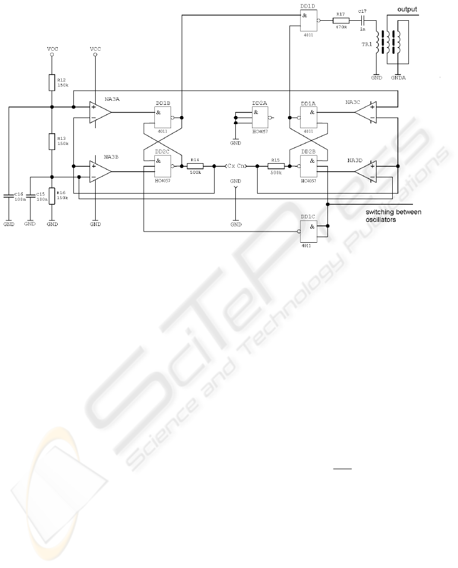
simplified schematic diagram of the oscillators is

shown in Fig. 2. Output signal of the running

oscillator is led via serial combination of the

capacitor and resistor to a primary winding of a

signal transformer. Serial resistor limits flowing

surge current when the logic output is changed.

Unfortunately, restriction of an exciting current

leads to extension of the rising and falling edge of

the transmitted signal. Serial capacity prevents bias

direct current from passing the transformer, thus

protects the transformer against overloading. The

output frequency of the oscillators can be calculated

using a simple equation

out

= ,

(1)

where R is value of reference resistor 500 kΩ and C

represents the measured capacity.

2.2 DC-DC Changer

The DC-DC changer with a transformer was

designed to supply the oscillators. The transformer

provides galvanic separation. In reality, construction

of the switched changer was the only one possible

solution and efficiency better than 50 % was

achieved. The circuitry of the changer consists of a

minimum component and is driven by an embedded

microcontroller. Unfortunately, the feedback cannot

Figure 2: Simplified schematic diagram of galvanically separated oscillators.

SMART DIFFERENTIAL PRESSURE SENSOR

245

be used because it leds to increased power

consumption.

2.3 Measurement Principle

The measurement is based on counting of 255

periods of the measured signal. Microcontroller

system clock is used as a sampling signal. Quiescent

frequency of the oscillators is set to 4.5 kHz. The

microcontroller counts 255 periods in 56 ms. Thus

total measurement time is 112 ms. These

calculations are not correct because the pair of

oscillators are not really identical, but even if real

measurement can be faster or slower, complete

measurement time is constant. This attribute is given

by design of the differential pressure sensor. The

measurement algorithm is implemented in the

microcontroller as follows: Counter/Timer0 (C/T0)

is configured as an 8-bit counter (it means 255

period of input signal). The Counter/Timer1 (C/T1)

runs as a 16-bit timer with 125 kHz clock before the

counting is allowed. The low system frequency of

the microcontroller significantly reduces power

consumption [3]. But minimal 1 MHz of the system

frequency is needed to suppose desired measurement

accuracy. Due to when 253 periods are counted the

microcontroller is over-clocked to 2 MHz. The value

in C/T1 is stored for next processing and C/T1 is

cleared. When the 255 periods are counted, the

interrupt is called and value in C/T1 is red. This

value reflects the measured capacity. With no

pressure the counter counts approximately 112 000

pulses from each oscillator. By using equation

2log

log

n =

(2)

where x represents numbers of levels and n is a bit

resolution, we can calculate that we can measure

oscillator frequencies with more than 16-bit

resolution.

This accuracy is adequate. For effective

processing of the measured values, the working

variable A(p) is evaluated. Variable A(p) represents

uncorrected digital pressure

)(

−

= ,

(3)

where f

and f

are measured frequencies of

oscillator output signals. At next stage the working

variable A(p) is calibrated using non-linear

corrections by hi-order polynomial. The calibration

provides linear response of the output value to the

pressure. The calibrated output value presents the

digital pressure and is set in specified units (bar,

kPa, etc.). After all linearization and calibration

processes the value is sent via SPI to the second

microcontroller which provides transmitting into the

current loop.

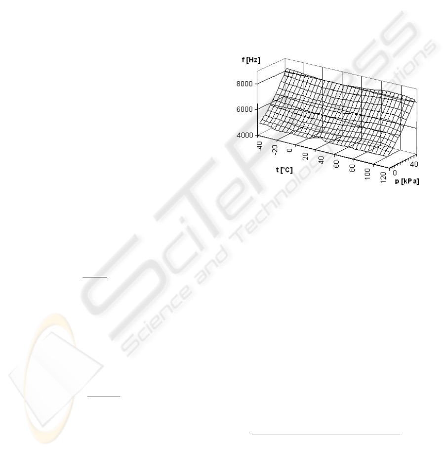
2.4 Corrections

Two corrections are calculated by the embedded

microcontroller. At first, the linearization, offset

calibration and gain correction are calculated. Next,

the temperature dependence of the measuring

electronics is compensated. Fig. 3 shows enumerated

dependencies in a 3D graph.

Figure 3: The oscillator output frequency dependence on

pressure and temperature.

There are a few calibration methods for example

lookup tables but these methods are usually of a high

cost and time consuming [2]. The polynomial of

fifth to eighth order is used for calibration of the

variable A(p). The basic form of the polynomial is

xaxaxaay ++++= ..

210

(4)

The Lagrange’s polynomial is used for calculation of

the calibration constants. The Lagrange’s

polynomial is the lowest order polynomial which

goes through specified values [4]. The Lagrange’s

polynomial can be calculated by

∑

)(

(5)

where

(

)

(

)

(

)( ) ( )

()( )( )( )( )

niiiiiii

nii

xxxxxxxxxx

−−−−−

+−

......

1121

(6)

The calibration data is stored in FRAM embedded

on the oscillator board.

ICINCO 2007 - International Conference on Informatics in Control, Automation and Robotics

246

2.5 HART Protocol

For communication over the 4 - 20 mA current loop,

the HART protocol is used [1]. Signal current

modulation is provided by the second

microcontroller. Transmitting is done using

controlled loading. The regulated loading circuitry is

very simple and consists of an NPN type bipolar

transistor with a grounded emitter and a driving DA

converter. Current consumption is minimized thanks

to simplicity of the regulated loading.

3 RESULTS

After design, assembly and programming of the

microcontroller real measurements were done. The

frequencies of the oscillators, working variable A

and digital pressure values were logged. These

values were logged for many different pressures

over the whole sensor range. From the measured

data the bias noise was figured out by equation

minmax

max

−

= ,

(7)

where ΔN

max

represents the maximal deviation from

the mean value of a few samples for a specified

pressure in the whole measuring range, N

max

is value

of the output with maximal pressure and N

min

value of the output with no pressure.

The bias noise in the whole measuring range was

only 0.82 ‰. By conversion of the bias noise to the

bit resolution the 13.57 effective bit resolution was

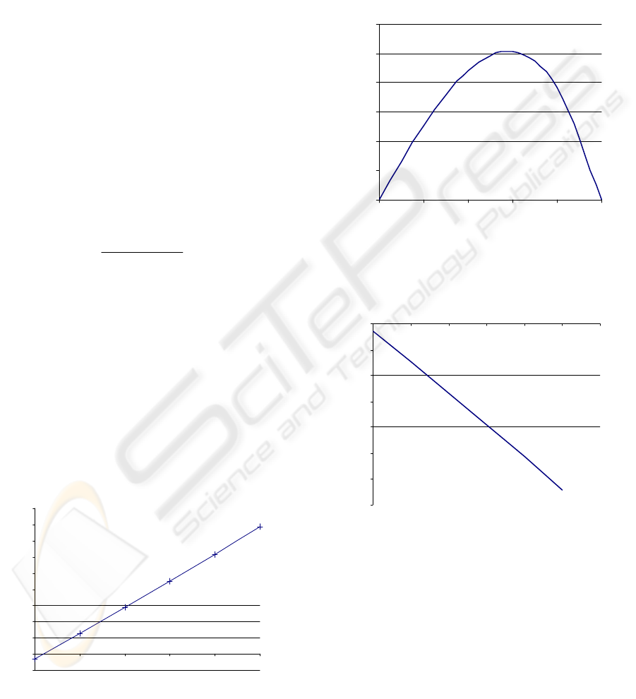
achieved. The linearity degree of the working

variable which determines order of the correction

polynomial is very important. The dependence of the

variable A(p) on pressure is shown in Fig. 4.

Figure 4: Dependence of the measured output on the

pressure.

We can observe deviations of the measured

waveform in Fig. 5.

And finally, deviation of the corrected

waveform is shown in Fig. 6, after calculating of the

Lagrange polynomial constants and their application

from the linear waveform.

Figure 5: Deviations of the measured waveform.

Figure 6: Deviations of the calibrated waveform.

4 CONCLUSIONS

A smart differential capacity pressure sensor was

designed and assembled. The system consists of

three parts – oscillators, processing microcontroller

and HART modulator. Ultra low-power devices and

special measuring algorithm in microcontroller were

used to reduce power consumption bellow 3.5 mA.

The Lagrange polynomials were applied to calculate

-0,05

0,05

0,1

0,15

0,2

0,25

0,3

0,35

0,4

0,45

0 1020304050

p [kPa]

x [-]

0,001

0,002

0,003

0,004

0,005

0,006

0 1020304050

p [kP a]

[-]

-0,00014

-0,00012

-0,0001

-0,00008

-0,00006

-0,00004

-0,00002

0 102030405060

p [kPa]



Ak [-]

SMART DIFFERENTIAL PRESSURE SENSOR

247

the measured values calibration. It improves

linearity more than ten times.

ACKNOWLEDGEMENTS

The research has been supported by the Czech

Ministry of Education within the framework of the

Research Program MSM0021630503 MIKROSYN,

by the Czech Grant Agency in projects GACR

102/03/0619 and GACR 102/03/H105, and by the

Ministry of Industry and Commerce in projects FF-

P/112 and FT-TA/050.

REFERENCES

HART communication foundation (2007) HART

specification,

http://www.hartcomm2.org/hart_protocol/protocol/har

t_specifications.html

Kouider, M. Nadi, M. and Kourtiche D. (2003) Sensors

Auto-calibration Method - Using Programmable

Interface Circuit Front-end, SENSORS 2003, ISSN

1424-8220

Holberg, A.M. and Seatre A. (2006) Innovative

Techniques for Extremely Low Power Consumption

with 8-bit Microcontrollers, ATMEL White Paper

Mori, H. and Yamada S. (2003) Continuation Power Flow

with the Nonlinear Predictor of the Lagrange’s

Polynomial Interpolation Formula, IEE Japan

ICINCO 2007 - International Conference on Informatics in Control, Automation and Robotics

248