ZISC Neural Network Base Indicator for Classification
Complexity Estimation
Ivan Budnyk, Abdennasser Сhebira and Kurosh Madani
Images, Signals and Intelligent Systems Laboratory (LISSI / EA 3956)
PARIS XII University, Senart-Fontainebleau Institute of Technology
Bat.A, Av. Pierre Point, F-77127 Lieusaint, France
Abstract. This paper presents a new approach for estimating task complexity
using IBM© Zero Instruction Set Computer (ZISC ©). The goal is to build a
neural tree structure following the paradigm “divide and rule”. The aim of this
work is to define a complexity indicator-function and to hallmark its’ main fea-
tures.
1 Introduction
In this paper, we present the key point of a modular neural tree structure used to solve
classification problems. This modular tree structure called Tree Divide To Simplify
(T-DTS) is based on the divide to conquer paradigm [1].
Complexity reduction is the
key point on which the presented modular approach acts. Complexity reduction is
performed not only at problem’s solution level but also at processing procedure’s
level. The main idea is to reduce the complexity by splitting a complex problem into a
set of simpler problems: this leads to “multi-modeling" where a set of simple models
is used to sculpt a complex behavior. Thus, one of the foremost functions to be per-
formed is the complexity estimation. The complexity estimation approach we present
in this paper is based on a neurocomputer [2]. Before describing the proposed ap-
proach, we present in the second section T-DTS paradigm and then the IBM© Zero
Instruction Set Computer (ZISC®) tool. In the third section we propose a new ap-
proach for complexity estimation. We validate our approach with an academic
benchmark problem and study the proposed indicator function’s properties. Final
section presents conclusion and further perspectives of the presented work.
2 Applied Systems
In a very large number of cases dealing with real world dilemmas and applications
(system identification, industrial processes, manufacturing regulation, optimization,
decision, pattern recognition, systems, plants safety, etc), information is available as
data stored in files (databases etc…) [3]. So, efficient data processing becomes a chief
condition to solve problems related to above-mentioned areas.
Budnyk I., Ð ˛ahebira A. and Madani K. (2007).
ZISC Neural Network Base Indicator for Classification Complexity Estimation.
In Proceedings of the 3rd International Workshop on Artificial Neural Networks and Intelligent Information Processing, pages 38-47
DOI: 10.5220/0001635600380047
Copyright
c
 SciTePress

An issue could be model complexity reduction by splitting a complex problem into a
set of simpler problems: multi-modeling where a set of simple models is used to
sculpt a complex behavior ([4] and [5]). For such purpose a tree-like splitting process,
based on complexity estimation, divides the problem’s representative database on a
set of sub-databases, constructing a specific model (dedicated processing module) for
each of obtained sub-databases. That leads to a modular tree-like processing architec-
ture including several models.
2.1 Neural Tree Modular Approach
In order to deal with real word problem, we have proposed a modular approach based
on divide and conquer paradigm ([1], [3]). In this approach, Tree Divide To Simplify
or T-DTS, we divide a problem in sub problems recursively and generate a neural tree
computing structure. T-DTS and associated algorithm construct a tree-like evolution-
ary neural architecture automatically where nodes are decision units, and leafs corre-
spond to neural based processing units ([5], [6], [7]).
Processing Results
Structure Construction
Learning Phas
e
Feature Space Splitting
NN based Models Generation
Preprocessing (Normalizing,
Removing Outliers, Principal
Component Analysis)
(PD) - Preprocessed Data Targets (T)
Data (D), Targets (T)
P – Prototypes Neural Network Trained Parameters
Operation Phase
Complexity
Estimation
Module
Fig. 1. General bloc diagram of T-DTS.
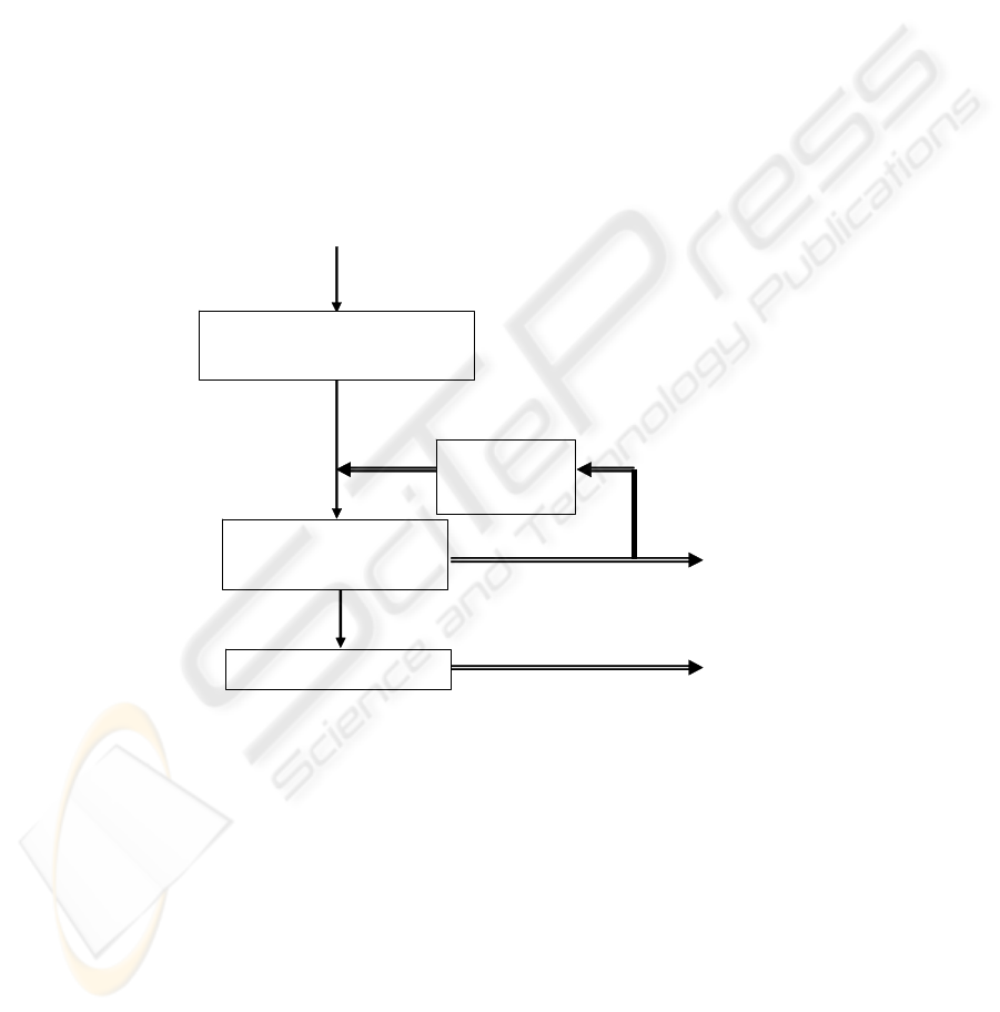
T-DTS includes two main operation modes. The first is the learning mode, when
T-DTS system decomposes the input database and provides processing sub-structures
and tools for decomposed sets of data. The second mode is the operation mode. Fig-
ure 1 gives the general bloc diagram of T-DTS operational steps. As shows this fig-
ure, T-DTS could be characterized by four main operations: “data pre-processing”,
“learning process”, “generalization process” and complexity estimation module. The
tree structure construction is guided mainly by the complexity estimation module.
This module introduces a feedback in the learning process and control the tree com-
puting structure. The reliability of tree model to sculpt the problem behavior is asso-
39

ciated mainly to the complexity estimation module. This paper focuses on this aspect
and proposes a new approach based on a neurocomputer. In the following sub-section
we describe ZISC® neurocomputer.
2.2 IBM(c) ZISC® Neurocomputer
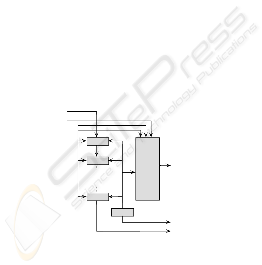
ZISC® neurocomputer is a fully integrated circuit based on neural network designed
for recognition and classification application which generally required supercomput-
ing. IBM ZISC-036 ([2], [5], [8]) is a parallel neural processor based on the RCE
(Reduced Coulomb Energy algorithm automatically adjusts the number of hidden
units and converges in only few epochs. The intermediate neurons are added only
when it is necessary. The influence field is then adjusted to minimize conflicting
zones by a threshold) and KNN algorithms (The k-nearest neighbor algorithm -
method for classifying objects based on closest training examples in the feature space.
k-NN is a type of instance-based learning, or lazy-learning where the function is only
approximated locally and all computation is deferred until classification).
Each chip is able to perform up to 250 000 recognitions per second ZISC® is the
implementation of the RBF-like (Radial Basic Function) model [9]. RBF approach
could be seen as mapping an N-dimensional space by prototypes. Each prototype is
associated with a category and an influence field. ZISC® system implements two
kinds of distance metrics called L1 and LSUP respectively. The first one (L1) corre-
sponds to a polyhedral volume influence field and the second (LSUP) to a hyper-
cubical one.
neuron 1
neuron 2
neuron 36
redrive
controls
address
data
[8]
[6]
[16]
I/O bus [30]
daisy chain i
n
[1]
logic
[4]
[21]
[1]
daisy chain out
inter Zisc communication bus
decision
output
Fig. 2. IBM ZISC-036 chip’s bloc diagram.
ZISC® neuron is an element, which is able:
40

• to memorize a prototype composed of 64 components, the associated category,
an influence field and a context,
• to compute the distance, based on the selected norm (norm L1 or LSUP) be-
tween its memorized prototype and the input vector,
• to compare the computed distance with the influence fields,
• to interact with other neurons (in order to find the minimum distance, category,
etc.),
• to adjust its influence field (during learning phase).
Fig 2 shows the bloc-diagram of an IBM© ZISC® chip. The next section present
the complexity estimation approach based on such neurocomputer’s capabilities.
3 Complexity Estimation Approach
The aim of complexity estimation is to check and measure the difficulty of a classifi-
cation task, before proper processing. Classification complexity estimation is used to
understand the behavior of classifiers. The most famous classification methods are
based on Bayes error, the theoretical probability of classification error. However it is
well known that Bayes error is difficult to compute directly. Significant part of com-
plexity estimation methods is related to Bayes error estimation. There are two general
ways to estimate Bayes error:
• indirectly [10] by proposing a measure which is a lower or higher bound of it
but easier to compute than direct estimation,
• Bayes error estimation by non-parametric method and show the relation to
Bayes error [11]. Other methods use space partitioning [12].
We deal with classification problems. We suppose that a database compounded of
a collection of m objects associated to labels or categories is available. To estimate
such database complexity we use the ZISC® as a classification tool. The goal we
want to reach is not to build a classifier for this problem, but to estimate the prob-
lems’ difficulty. We first used the ZISC® neurocomputer to learn this classification
problem using the associated database. Then we estimate the task complexity by
analyzing the generated neural network structure. We expect that a more complex
problem will involve a more complex structure. The simplest neural network structure
feature is the number n of neurons created during the learning phase. The following
indicator is defined, where n is a parameter that reflects complexity:
m
n
Q =
,
0,1 ≥≥ nm
(1)
We suppose that there exists some function n = g(.) that reflects problem com-
plexity. The arguments of this function may be the signal-to-noise ratio, the dimen-
sion of the representation space, boundary non-linearity and/or database size.
In a first approach, we consider only g(.) function’s variations according to m
axis: g(m).
We suppose that our database is free of any incorrect or missing information.
On the basis on g(m), a complexity indicator is defined as follow:
41

m
mg
mQ
i
i
)(
)( =
0)(,1, ≥≥ mgm
i
(2)
We expect that for the same problem, as we enhance m, the problem seem to be
less complex: more information reduces problem ambiguity. On the other hand, for
problems of different and increasing complexity, Q
i
indicator should have a higher
value. In order to check the expected behavior of this indicator function, we have
defined an academic and specific benchmark presented in the following sub-section.
3.1 Academic Benchmark Description
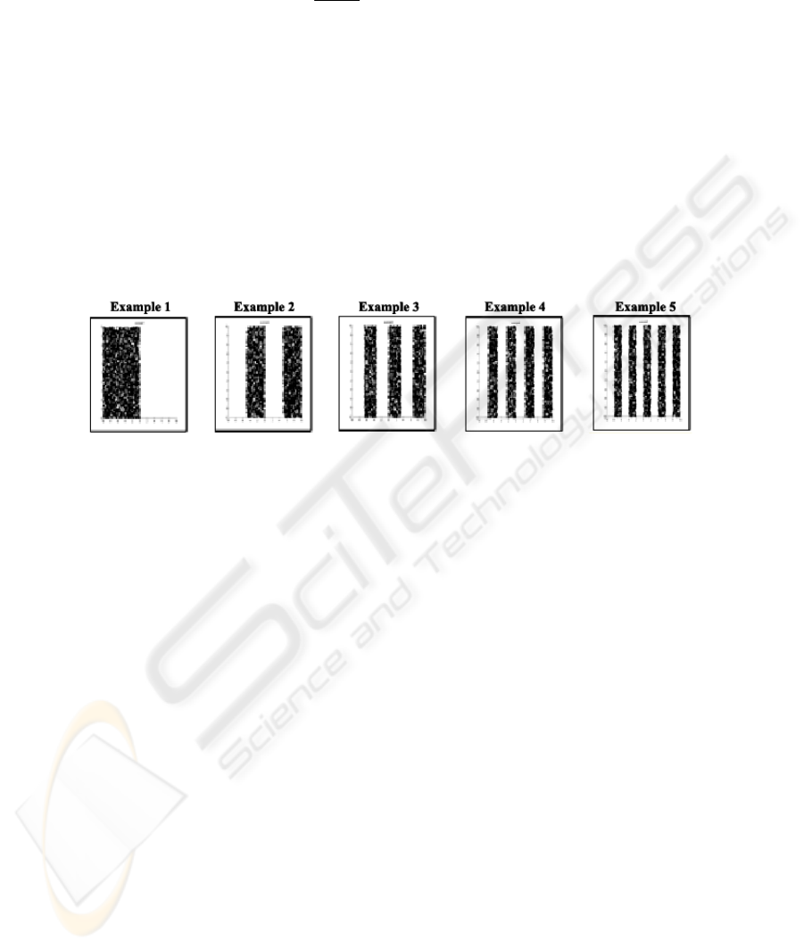
Basically we construct 5 databases representing a mapping of a restricted 2D space to
2 categories, (Fig. 3). Each pattern was divided into two and more equal striped sub-
zones, each of them belonging to the categories 1 or 2 alternatively.
Fig. 3. Test patterns.
In learning mode, we create samples using randomly generated points with coor-
dinates (x,y). The number of samples m, in our case of uniform random distribution,
naturally has an influence on the quality of the striped zones (categories) demarca-
tion. According to the value of the first coordinate x, and according to the amount of
the striped sub-zones, the appropriate category c is assigned to the sample, and such
structure (x
j
,y
j
, c
j
) sends to neurocomputer on learning.
The second mode is a classification or in other words real testing of the generaliz-
ing ZISC® neurocomputer abilities. We again, randomly and uniformly, generate m
samples and their associated category. Getting classification statistics, we compute
the indicator-function Q
i
.
3.2 Results
The testing has been performed within:
• 2 IBM(c) ZISC® modes (LSUP/L1),
• 5 different databases with increasing complexity,
• 8 variants of m value (50, 100, 250, 500, 1000, 2500, 5000, 10000).
For each set of parameters, tests are repeated 10 times in order to get statistics and
as stated to check the deviations and to get average. Totally, 800 tests have been per-
formed.
42

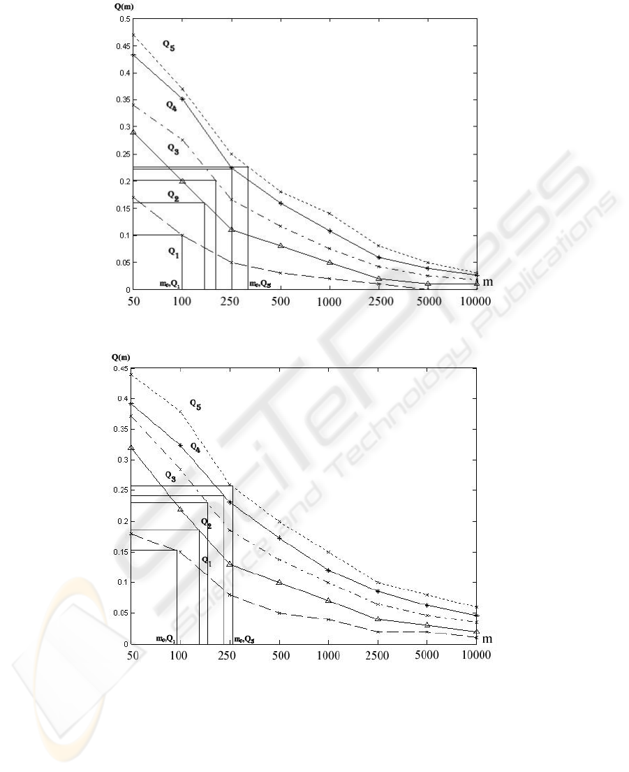
Fig. 4. LSUP ZISC’s mode, Q
i
(m).
Fig. 5. L1 ZISC’s mode, Q
i
(m).
Fig. 4 and Fig. 5 show the charts of Q
i
where i is the database index or pattern in-
dex. We expect that Q
5
for 10 sub-zones reaches a higher value than Q
1
. Intuitively the
problem corresponding to classification of 10 stripped zones (Q
5
) is more complex
than for 2 (Q
1
).
43

The chart analysis suggests that exists a point(s) m
j
such as:
0)(
)(
2
2
=
∂
∂
ji
mQ
m
(3)
At such point m
j
we have the following propreties:
0)(
)(
,0)(
)(
);(:0,1
2
2
2
2
>
∂
∂
⇒>∀<
∂
∂
⇒
−
∈
∀
>∃≥∀
jijji
jjjj
mQ
m
mmmQ
m
mmmm
ε
ε
(4.1)
or
0)(
)(
,0)(
)(
);(:0,1
2
2
2
2
<
∂
∂
⇒>∀>
∂
∂
⇒
−
∈
∀
>∃≥∀
jijji
jjjj
mQ
m
mmmQ
m
mmmm
ε
ε
(4.2)
It means that there exists one or more points m
j
where the second derivative of Q
i
changes its sign. Then we are interesting in m
0
defined by:
kj
kkj
mmm
mmmmm
<<<<
=
=
.....
,),...,..,max(
1
10
(5)
Where k is the number of points m
j
.
After polynomial approximation for 2 different ZISC’s modes we compute the
coefficients of complexity Q
i
(m
0
). Table 1 represents the summary of the obtained
results described on the Figures 4 and 5
Table 1. Coefficients of complexity for DNA sequences recognition.
Main characteristic of the point m
0
is:
constmQmmm
i
→⇒
+
∞→>∀ )(:
0
(6)
In our case const = 0 , in general not obviously const = 0. The feature of the second
derivative sign changing is also a characteristic of success rate of the classification
(Fig. 6 and Fig. 7).That supports the idea of the strong influence second derivate fea-
ture has on the complexity estimation task. That fact turn a look on the problems not
LSUP L1
ZISC’s mode
m
0
Q
i
(m
0
) m
0
Q
i
(m
0
)
Example 1 100 0.154 88 0.151
Example 2 170 0.182 168 0.177
Example 3 190 0.233 186 0.229
Example 4 235 0.240 229 0.239
Example 5 265 0.261 254 0.254
44

from the quantity side of complexity, but allows us to make a transitional step on the
quality level. It is clearly seen that in our pattern examples, complexity of the classifi-
cation is lying in the range from Example 1 (2 zones, the easiest one) till Example 5.
Analysis of the plots m
0,Q1
(Example 1) till m
0,Q5
(Example 5) for related classification
tasks implies the following property:
54321
,0,0,0,0,0 QQQQQ
mmmmm
<
<
<
<
(7)
In our particular case
)()()()()(
0504030201
mQmQmQmQmQ
<
<
<
<
(8)
In our experimental validations, the relation (6) (giving the limit of Q
i
(m) when m
becomes + ∞) can be interpreted as the case where m is large comparing to m
0
mean-
ing that the additional new data doesn’t change the dynamic of the classification tasks.
In other words this signifies that situation becomes more predictable regarding indica-
tors’ evolution (Fig 4 and Fig 5) and the classification rates (Fig 6 and Fig 7).
Fig. 6. Success rates of patterns’ classification. Example 1 – 5. LSUP ZISC’s mode.
45

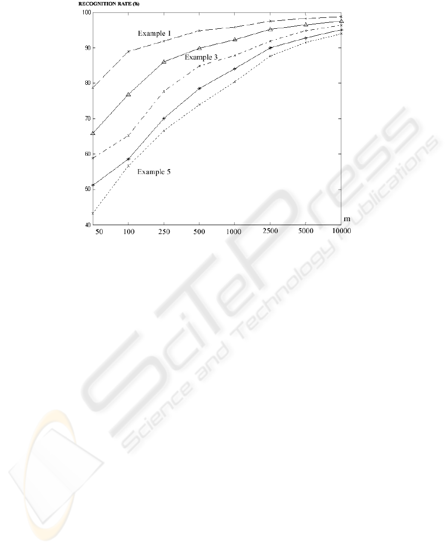
Fig. 7. Success rates of patterns’ classification. Example 1 – 5. L1 ZISC’s mode.
On the other hand, one can consider a particular value of m (an interesting value is
m
0
for which the second derivative of Q
i
(m) changes the sign) making Q
i
(m
0
) acting as
a “complexity coefficient”. In our case, Q
i
(m
0
) acts as a “checkpoint” evaluating the
“stability of the classification process”. The increase of m
0
stands for the classification
task’s complexity increasing.
4 Conclusions
In this paper we describe a new method for complexity estimation and propose a
constructed Q(m) – indicator function. This approach is based on the ZISC neuro-
computer. The complexity indicator is extracted from some pertinent neural network
structure parameters and specifically in this paper from the number of neuron in the
structure. More complex structures are related to more complex problems. The pre-
sented concept have been implemented on IBM© ZISC-036 ® massively parallel
neurocomputer validated using a two-classes set of classification academic bench-
marks with increasing complexity. First investigation of the second derivative sign
behavior of the proposed complexity indicator allows to exhibit some interesting
properties.
Perspectives of this work will be a formal description of the defined complexity
indicator, the specification of other pertinent parameters and the study of their proper-
ties. We are also working on the validation of this theoretical approach to complexity
46

evaluation of a real-word problem in the medical area: DNA patterns classification
(recognizing given a sequence of DNA the boundaries between exons and introns).
References
1. Bouyoucef, E., Chebira A., Rybnik, M., Madani, K.: 2005. Multiple Neural Network
Model Generator with Complexity Estimation and self-Organization Abilities. Interna-
tional Scientific Journal of Computing, ISSN 1727-6209, vol.4, issue 3, pp.20-29.
2.
Laboratory IBM France: May 15, 1998, ZISC® 036 Neurons User’s Manual, Version 1.2,
Component Development.
3.
Madani, K., Rybnik, M., Chebira A.: 2003. Data Driven Multiple Neural Network Models
Generator Based on a Tree-like Scheduler, LNCS series, Edited by: Mira, J., Prieto A., -
Springer Verlag, ISBN 3-540-40210-1, pp. 382-389.
4.
Jordan, M. I., Xu, L.: 1995. Convergence Results for the EM Approach to Mixture of Ex-
perts Architectures, Neural Networks, Vol. 8, N° 9, pp 1409-1431, Pergamon, Elsevier.
5.
Madani, K., Chebira, A.: 2000. A Data Analysis Approach Based on a Neural Networks
Data Sets Decomposition and it’s Hardware Implementation, PKDD 2000, Lyon, France.
6.
Tremiolles, G. De: March 1998. Contribution to the theoretical study of neuro-mimetic
models and to their experimental validation: a panel of industrial applications, Ph.D. Re-
port, University of PARIS XII.
7.
Tremiolles, G. De, Tannhof, P., Plougonven B., Demarigny C., Madani, K.: 1997. Visual
Probe Mark Inspection, using Hardware Implementation of Artificial Neural Networks, in
VLSI Production, LNCS - Biological and Artificial Computation : From Neuroscience to
Technology, Ed.: Mira, J., Diaz R. M., Cabestany J., Springer Verlag Berlin Heidelberg,
pp. 1374-1383.
8.
Laboratory IBM France: February 1995. ISC/ISA ACCELERATOR card for PC, User
Manual, IBM France.
9.
Park, J., Sandberg, J.W.: 1991. Universal approximation using radial basis functions net-
work, Neural Computation, vol. 3. pp. 246-257.
10.
Lin, J.: 1991. Divergence measures based on the Shannon entropy, IEEE Transactions on
Information Theory, 37(1):145-151.
11.
Parzen, E.: 1962. On estimation of a probability density function and mode, Annals of
Math. Statistics, vol. 33, pp. 1065-1076.
12.
Kohn, A., Nakano, L.G., Mani, V.: 1996. A class discriminability measure based on feature
space partitioning, Pattern Recognition, 29(5):873-887.
47