SIMULTANEOUS REGISTRATION AND CLUSTERING FOR
TEMPORAL SEGMENTATION OF FACIAL GESTURES FROM
VIDEO
Fernando De la Torre, Joan Campoy, Jeffrey F. Cohn and Takeo Kanade
Robotics Institute, Carnegie Mellon University, Pittsburgh, USA
Keywords:
Facial expression analysis, Clustering, Facial Gesture, Learning, Temporal segmentation.
Abstract:
Temporal segmentation of facial gestures from video sequences is an important unsolved problem for auto-
matic facial analysis. Recovering temporal gesture structure from a set of 2D facial features tracked points is a
challenging problem because of the difficulty of factorizing rigid and non-rigid motion and the large variability
in the temporal scale of the facial gestures. In this paper, we propose a two step approach for temporal seg-
mentation of facial gestures. The first step consist on clustering shape and appearance features into a number
of clusters and the second step involves temporally grouping these clusters.
Results on clustering largely depend on the registration process. To improve the clustering/registration, we
propose a Parameterized Cluster Analysis (PaCA) method that jointly performs registration and clustering.
Besides the joint clustering/registration, PaCA solves the rounding off problem of existing spectral graph
methods for clustering. After the clustering is performed, we group sets of clusters into facial gestures. Several
toy and real examples show the benefits of our approach for temporal facial gesture segmentation.
1 INTRODUCTION
Temporal segmentation of facial gestures from video
sequences is an important unsolved problem towards
automatic facial interpretation. Recovering tempo-
ral gesture structure from a set of 2D facial features
tracked points is a challenging problem because of
the difficulty of factorizing rigid and non-rigid mo-
tion and the variability of temporal scales for differ-
ent facial gestures. This problem is particulary hard if
the sequence contains subtle expression changes and
strong pose changes (most real interesting video se-
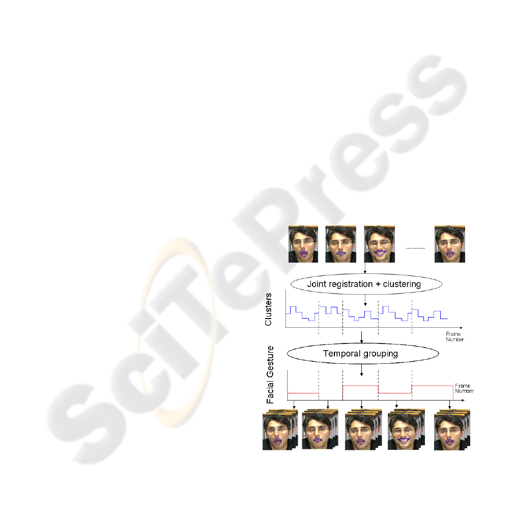
quences). In this paper, we propose a two step ap-
proach to temporal segmentation of facial gestures.
The first step groups the shape and appearance fea-
tures of facial features into a given number of clusters.
The second step finds the temporal grouping of these
clusters (see fig. 1).
A key for the success of the clustering relies on the
registration step. If the tracker do not explicitly track
with a 3D model is usually hard to decouple rigid and
non-rigid motion. In this paper, we propose Para-
meterized Cluster Analysis (PaCA), that jointly per-
forms registration and clustering. Once the clustering
is done, we propose a simple but effective way of dis-
Figure 1: Temporal segmentation of facial gestures.
covering temporal structure in the set of clusters. Ad-
ditionally, a new matrix formulation for clustering is
introduced that enlightens connections between clus-
tering methods.
110
De la Torre F., Campoy J., F. Cohn J. and Kanade T. (2007).
SIMULTANEOUS REGISTRATION AND CLUSTERING FOR TEMPORAL SEGMENTATION OF FACIAL GESTURES FROM VIDEO.
In Proceedings of the Second International Conference on Computer Vision Theory and Applications - IU/MTSV, pages 110-115
Copyright
c
 SciTePress

2 PREVIOUS WORK
There has been quite substantial research efforts de-
voted to facial expression analysis over the past few
years. Most of the work focus on tracking (Zhao and
Chellappa, 2006), facial expression recognition or ac-
tion units recognition (Lucey et al., 2006; Cohn et al.,
2006). Little attention has been paid to the problem
of temporal segmentation of facial gestures that can
greatly benefit the recognition process. Exception is
the pioneering work of Mase and Pentland (Mase and
Pentland, 1990) that shows how zeros of the velocity
of the facial motion parameters were found to be use-
ful for the temporal segmentation and its applications
to lip reading. Recently, Joey (Hoey, 2001) present
a Multilevel Bayesian network for learning the dy-
namics of facial expression. In related work, Irani
and Zelnik (Zelnik-Manor and Irani, 2004) propose a
modification of factorization algorithms for structure
from motion to provide temporal clustering of non-
rigid motion.
Most previous work assumes an accurate registra-
tion process before the segmentation step. Accurate
registration of the non-rigid facial features is still an
open research problem (Zhao and Chellappa, 2006),
in particular decoupling rigid and non-rigid motion
from 2D. Unlike previous research, in this paper we
propose an algorithm that jointly performs registra-
tion and clustering as a first step toward temporal seg-
mentation of facial gestures. Moreover, we develop a
simple but effective way to group these clusters into
temporally coherent chunks.
3 MATRIX FORMULATION FOR
CLUSTERING
In this section we review the state of the art in clus-
tering algorithms using a new matrix formulation that
enlightens the connection between several clustering
methods and suggests new optimization schemes for
spectral clustering.
3.1 K-means
K-means (MacQueen, 1967; Jain, 1988) is one of the
simplest and most popular unsupervised learning al-
gorithms to solve the clustering problem. Clustering
refers to the partition of n data points into c disjoint
clusters. k-means clustering splits a set of n objects
into c groups by maximizing the between-clusters
variation relative to within-cluster variation. That is,
k-means clustering finds the partition of the data that
is a local optimum of the following energy function:
J(µ
µ
µ
1
,...,µ
µ
µ
n
) =
∑
c
i=1
∑
j∈C
i
||d
j
− µ
µ
µ
i
||
2
2
where d
j
(see
notation
1
) is a vector representing the j
th
data point
and µ
µ
µ
i
is the geometric centroid of the data points for
class i. The optimization criteria in previous eq. can
be rewritten in matrix form as:
E
1
(M,G) = ||D −MG
T
||
F
(1)
sub ject to G1
c
= 1
n
and g
i j
∈ {0, 1}
where G ∈ ℜ
n×c
and M ∈ ℜ
d×c
. G is a dummy in-
dicator matrix, such that
∑
j
g
i j
= 1, g
i j
∈ {0,1} and
g
i j
is 1 if d
i
belongs to class C
j
, c denotes the number
of classes and n the number of samples. The columns
of D ∈ ℜ
d×n
contain the original data points, d is the
dimension of the data. Recall that the equivalence be-
tween the k-means error function and eq. 1 is only
valid if G strictly satisfies the constraints.
The k-means algorithm performs coordinate de-
scent in E
1
(M,G). Given the actual value of the
means M, the first step finds for each data point d
j
,
the g
j
such that one of the columns is one and the
rest 0 and minimizes eq. 1. The second step opti-
mizes over M = DG(G
T
G)
−1
, equivalent to compute
the mean of each cluster. Although it can be proven
that alternating these two steps will always terminate,
the k-means algorithm does not necessarily find the
optimal configuration over all possible assignments.
It typically runs multiple times and the best solution
is chosen. Despite these limitations, the algorithm is
used fairly frequently as a result of its ease of imple-
mentation and effectiveness.
Eliminating M, eq. 1 can be rewritten as:
E
2
(G) = ||D −DG(G
T
G)
−1
G
T
||
F
= tr(D
T
D)
−tr((G
T
G)
−1
G
T
D
T
DG) ≥
∑
min(d,n)
i=c+1
λ
i
(2)
where λ
i
are the eigenvalues of D
T
D. Min-
imizing eq. 2 is equivalent to maximizing
tr((G
T
G)
−1
G
T
D
T
DG). Ignoring the special struc-
ture of G and considering the continuous domain, the
optimum G value that optimizes eq. 2 is given by the
eigenvectors of the covariance matrix D
T
D and the er-
ror is E
2
=
∑
min(d,n)
i=c+1
λ
i
. A similar reasoning has been
reported by (Ding and He, 2004; Zha et al., 2001),
1
Bold capital letters denote a matrix D, bold lower-case
letters a column vector d. d
j
represents the j column of the
matrix D. d
i j
denotes the scalar in the row i and column
j of the matrix D and the scalar i-th element of a column
vector d
j
. All non-bold letters will represent variables of
scalar nature. diag is an operator that transforms a vector to
a diagonal matrix or takes the diagonal of the matrix into a
vector. ◦ denotes the Hadamard or point-wise product. 1
k
∈
ℜ
k×1
is a vector of ones. I
k
∈ ℜ
k×k
is the identity matrix.
tr(A) =
∑
i
a
ii
is the trace of the matrix A and |A| denotes
the determinant. ||A||
F
= tr(A
T
A) = tr(AA
T
) designates
the Frobenious norm of a matrix.
SIMULTANEOUS REGISTRATION AND CLUSTERING FOR TEMPORAL SEGMENTATION OF FACIAL
GESTURES FROM VIDEO
111

where they show that a lower bound of eq. 2 is given
by the residual eigenvalues. The continuous solution
of G lies in the c − 1 subspace spanned by the first
c−1 eigenvectors with highest eigenvalues (Ding and
He, 2004) of D
T
D.
3.2 Spectral Clustering
Spectral graph methods for clustering are popular be-
cause of ease of programming and because they ac-
complishes a good trade-off between achieved per-
formance and computational complexity. Recently,
(Dhillon et al., 2004; de la Torre and Kanade, 2006)
point out the connections between k-means and stan-
dard spectral graph algorithms, such as Normalized
Cuts (Shi and Malik, 2000), by means of kernel meth-
ods. The kernel trick is a standard way of lifting
the points of a dataset to a higher dimensional space,
where points are more likely to be linearly separable
(assuming that the right mapping is found). Let us
consider a lifting of the original points to a higher di-
mensional space, Γ = [ φ(d
1
) φ(d
2
) ··· φ(d
n
) ] where
φ is a high dimensional mapping. The kernelized ver-
sion of eq. 1 will be:
E
3
(M,G) = ||(Γ −MG
T
)W||
F
(3)
where we have introduced a weighting matrix W
for normalization purposes. Eliminating M =
ΓWW
T
G(G
T
WW
T
G)
−1
, it can be shown that:
E
3
∝ −tr((G
T
WW
T
G)
−1
G
T
WW
T
Γ
T
ΓWW
T
G) (4)
where Γ
T
Γ is the standard affinity matrix in Normal-
ized Cuts (Shi and Malik, 2000). After a change
of variable Z = G
T
W, the previous equation can be
expressed as E
3
(Z) ∝ −tr((ZZ
T
)
−1
ZW
T
Γ
T
ΓWZ
T
).
Choosing W = diag(Γ
T
Γ1
n
)
−0.5
the problem is
equivalent to solving the Normalized Cuts problem.
Observe that this formulation is more general since
it allows for arbitrary kernels and weights. Also, ob-
serve that the weight matrix could be used to reject
the influence of a pair of data points with unknown
similarity (i.e. missing data).
4 PARAMETERIZED CLUSTER
ANALYSIS
Good registration is critical for segmentation of sub-
tle facial gestures. However, decoupling the rigid and
non-rigid motion of the face is a challenging problem
even if 3D models are used. In this section, we pro-
pose PaCA that jointly performs clustering and reg-
istration and alleviates the registration problem for
clustering.
4.1 Energy Function for PaCA
The key idea of PaCA is to parameterize the shape
features Γ in the clustering function. This can be done
easily by relating the clustering problem to an error
function:
E
1
(A,G,M) = ||Γ − MG
T
||
F
(5)
Unlike previous section, Γ = φ(T(A,D)) =
[ φ(A
1
d
1
) φ(A
2
d
2
) · · · φ(A
n
d
n
) ] is a parameterized
version of the data that accounts for mis-registrations.
Each column in T(A,D) ∈ R
d×n
, t
i
represents the
warped shape A
i
d
i
, where A
i
is a linear transforma-
tion matrix with the motion parameters. φ is a generic
mapping, usually to a higher dimensional space. The
mapping can be infinite dimensional (e.g. Gaussian
kernel).
After optimizing over M = ΓG(G
T
G)
−1
, eq. 5 is
equivalent to:
E
2
(A,G) = ||Γ(A)(I −G(G
T
G)
−1
G
T
)||
F
=
tr

Γ(A)
T
Γ(A)(I − G(G
T
G)
−1
G
T
)

(6)
taking into account that (I − G(G
T
G)
−1
G
T
) is a
idempotent matrix. K(A) = Γ(A)
T
Γ(A) is the stan-
dard affinity matrix or kernel matrix, where each el-
ement in the case of exponential kernel is: k
i j
=
e
−
||A
i
D
i
−A
j
D
j
||
F
2σ
. Where A
i
is an affinity matrix of 4
(if translation is removed), 6 or 8 parameters. D
i
∈
R
(d/2)×n
is a data matrix, such that the first row con-
tains the x-coordinates and the second row contains
the y-coordinates.
4.2 Motion Models
In this paper, we will assume that in the video the face
of the subject is relatively far away from the camera
and that locally the eye region or mouth is a planar
surface. It is well known (Adiv, 1985) that the 2D
projected motion field of a 3D planar surface can be
recovered under orthographic projection (x = X and
y = Y ) by an affine model f(x, a), parameterized by
a = [a
1
a
2
... a
6
]
T
:
f(x,a) =

a
1
a
4

+

a
2
a
3
a
5
a
6

x − x
c
y − y
c

(7)
where x
c
= (x
c
,y
c
)
T
is the center position of the ob-
ject.
4.3 Solving the Optimization Problem
Assuming the matrix A is known, optimizing eq. 6
reduces to:
E
5
(G) ∝ tr((G
T
G)
−1
G
T
KG) (8)
VISAPP 2007 - International Conference on Computer Vision Theory and Applications
112

To impose non-negativity constraints in g
i j
, we para-
meterize G as the product of two matrices G = V ◦ V
(de la Torre and Kanade, 2006) and use a gradient de-
scent strategy to search for an optimum:
V
n+1
= V
n
− η
1
∂G(V
n
)
∂V
(9)
∂G(V
n
)
∂V
= (I
c
− G(G
T
G)
−1
G
T
)KG(G
T
G)
−1
◦ V
The major problem with the update of eq. 9 is
to determine the optimal η
1
. In our case, η
1
is deter-
mined with a line search strategy. To impose G1
c
= 1
n
in each iteration, the V is normalized to satisfy the
constraint. Because eq. 9 is prone to local minima,
we start from several random initial points and select
the solution with minimum error.
Assuming G is known optimizing w.r.t. A has
to minimize: E
3
(A) = tr

K(A)F

where, F = (I −
G(G
T
G)
−1
G
T
). To optimize w.r.t. A we use a linear
time algorithm that uses gradient descent. In the case
of exponential kernel,
A
n+1
= A
n
− η
2
∂E
2
∂A
(10)
∂E
∂A
i
= −
∑
n
j=1
f
ji
σ
e
−
||A
i
D
i
−A
j
D
j
||
F
2σ
(A
i
D
i
− A
j
D
j
)D
T
j
As before, η
2
is determined with a line search
strategy (Fletcher, 1987).
4.4 Initialization and Clustering
Features
Optimizing eq. 6 w.r.t A and G is a non-convex prob-
lem prone to local minima, that without a good initial-
ization is likely to get stuck into a bad minimum. To
give an initial estimate of the matrix K we compute
all possible pairwise affine distances between the set
of shape points and with this estimate optimize over
G. Observe that at this point K is symmetric but not
necessarily definite positive.
We assume that several facial features of the face
have been tracked using Active Appearance Models
(AAM) (Matthews and Baker, 2004) (see fig. 6).
Once the facial feature points have been tracked, we
use PaCA to jointly cluster and register the shape.
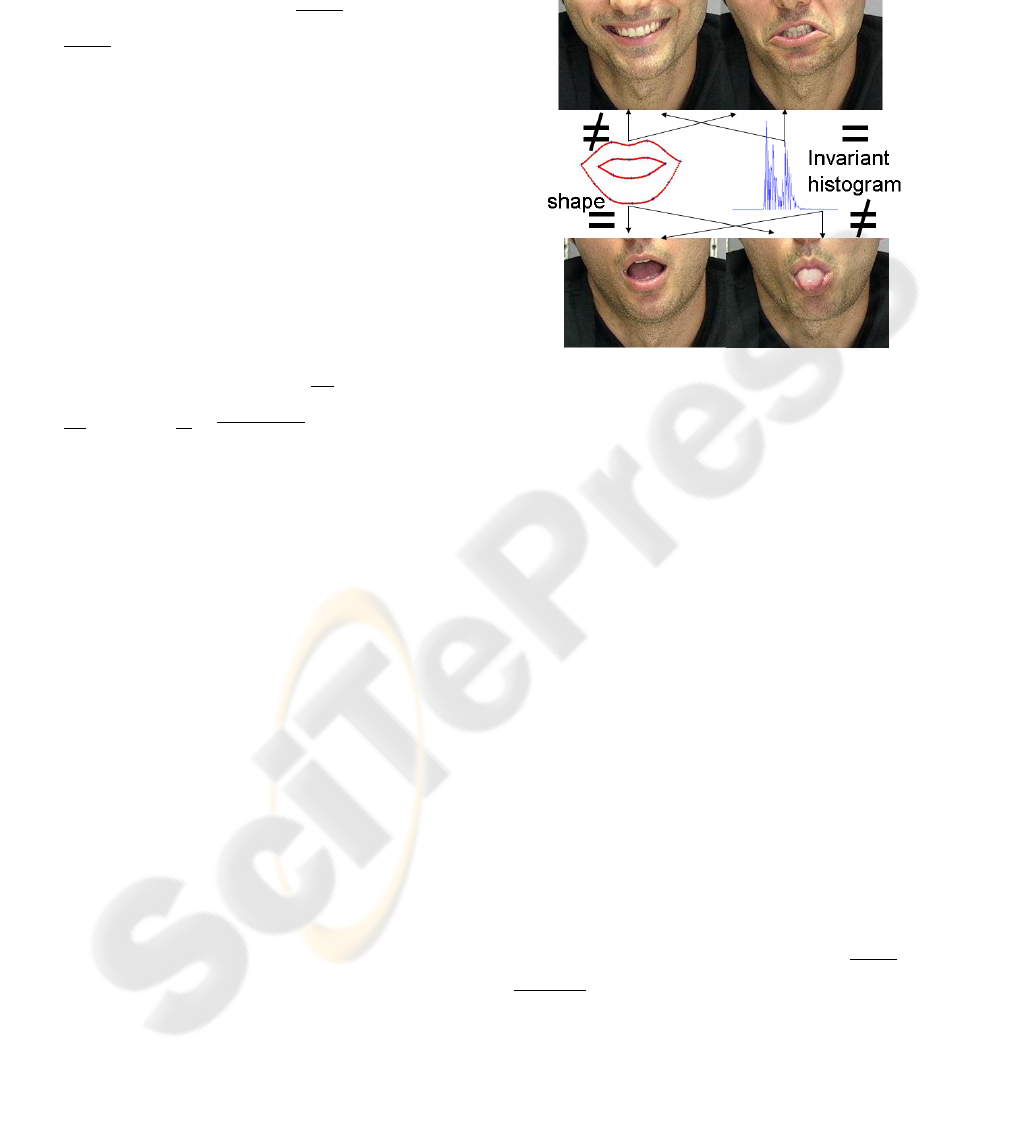
However, using only the shape as the only feature
is not very reliable for capturing subtle facial ges-
tures. For instance, we can have two completely dif-
ferent gestures with the same shape (see fig. 2 bot-
tom). To compensate for this effect, we also incor-
porate appearance features. The appearance features
are extracted by a geometric invariant histogram re-
cently introduced (Domke and Aloimonos, 2006). We
can decouple the effects of registration in the appear-
ance representation since the histogram proposed in
(Domke and Aloimonos, 2006) is invariant to per-
spective transformations (see fig. 2). During the
clustering process we over-sample the shape feaures
to achieve robustness against noise(see fig. 2).
Figure 2: Features used in temporal segmentation.
5 DISCOVERING TEMPORAL
CLUSTERS
Once the the facial features have been clustered into
coherent shape/appearance clusters, the goal is to
group the clusters into facial gestures. In this section,
we propose a simple but effective method to search
for temporal coherent clusters.
5.1 Removing Temporal Redundancy
In a first step, we automatically detect all neutral ex-
pressions (i.e. action unit 0-AU0) (Cohn et al., 2006)
since is usually the most common facial ”cluster” and
useful in many recognition tasks. The algorithm to
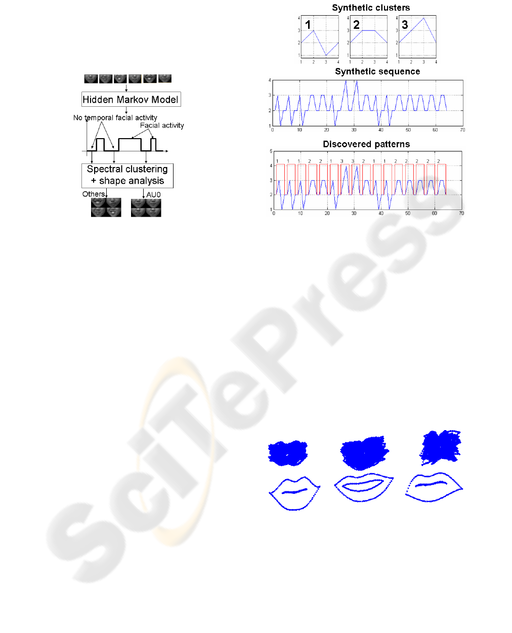
detect the AU0 works as follows. First, we compute
a normalized error between the shape/appearance at
time t and time t − 1. A two-state Hidden Markov
Model (HMM) is used to temporally segment the time
instants that contain appearance/shape changes. The
transition probabilities in the HMM are computed us-
ing a logistic regression function (i.e.
1
1+e
−βx
and
1
1+e
−β(x+τ)
), where β, τ are parameters computed from
the error histogram. To find a maximum a posteri-
ori solution, the standard Viterbi algorithm (dynamic
programming) is executed. In the state represent-
ing still configurations of the face there are exam-
ples of AU0 and examples of other AU that are sta-
tic for few frames. In the next step, we separate
SIMULTANEOUS REGISTRATION AND CLUSTERING FOR TEMPORAL SEGMENTATION OF FACIAL
GESTURES FROM VIDEO
113

these two cases by performing spectral clustering with
shape/appearance features. All the clusters such that
the average mean aperture of the mouth is smaller that
a threshold are classified as AU0. Fig 3 illustrates the
process.
Figure 3: Process to automatically detect AU0.
The second important step towards discovering
temporal clusters is to achieve temporal invariance to
the speed of the facial gesture. Towards this end, we
first remove all the consecutive clusters that are the
same and just the changes among consecutive clus-
ters will remain. After this process is done, the video
is reduced to about 10 − 20% its original length.
5.2 Temporal Correlation to Discover
Facial Gestures
Once we have simplified the temporal representation
of the video sequence, we are ready to find tempo-
ral patterns of different lengths in the video sequence.
Since we have substantially reduced the amount of
temporal data available, we use an exhaustive ap-
proach to search over all possible cluster sequences of
different lengths and in the sequence to find the same
temporal pattern.
The algorithm starts selecting long patterns (usu-
ally 8 − 9 clusters), and it searches over the whole se-
quence for peaks of the normalized correlation. All
the peaks that have normalized correlation 1 (i.e. is
the same pattern) are removed from the sequence,
later the rest of the patterns with smaller length are
iteratively discovered with the same approach.
Fig. 4 shows how the algorithm works in syn-
thetic data. We have made a sequence with three tem-
poral clusters of length 4 (fig. 4.a and 4.b). The al-
gorithm automatically discovers that there are 3 tem-
poral clusters and correctly identifies them.
Figure 4: a) 3 synthetic clusters b) synthetic sequence c)
Temporal clusters found with our algorithm.
6 EXPERIMENTS
In this section we report preliminary experiments with
synthetic and real data.
6.1 Synthetic Data
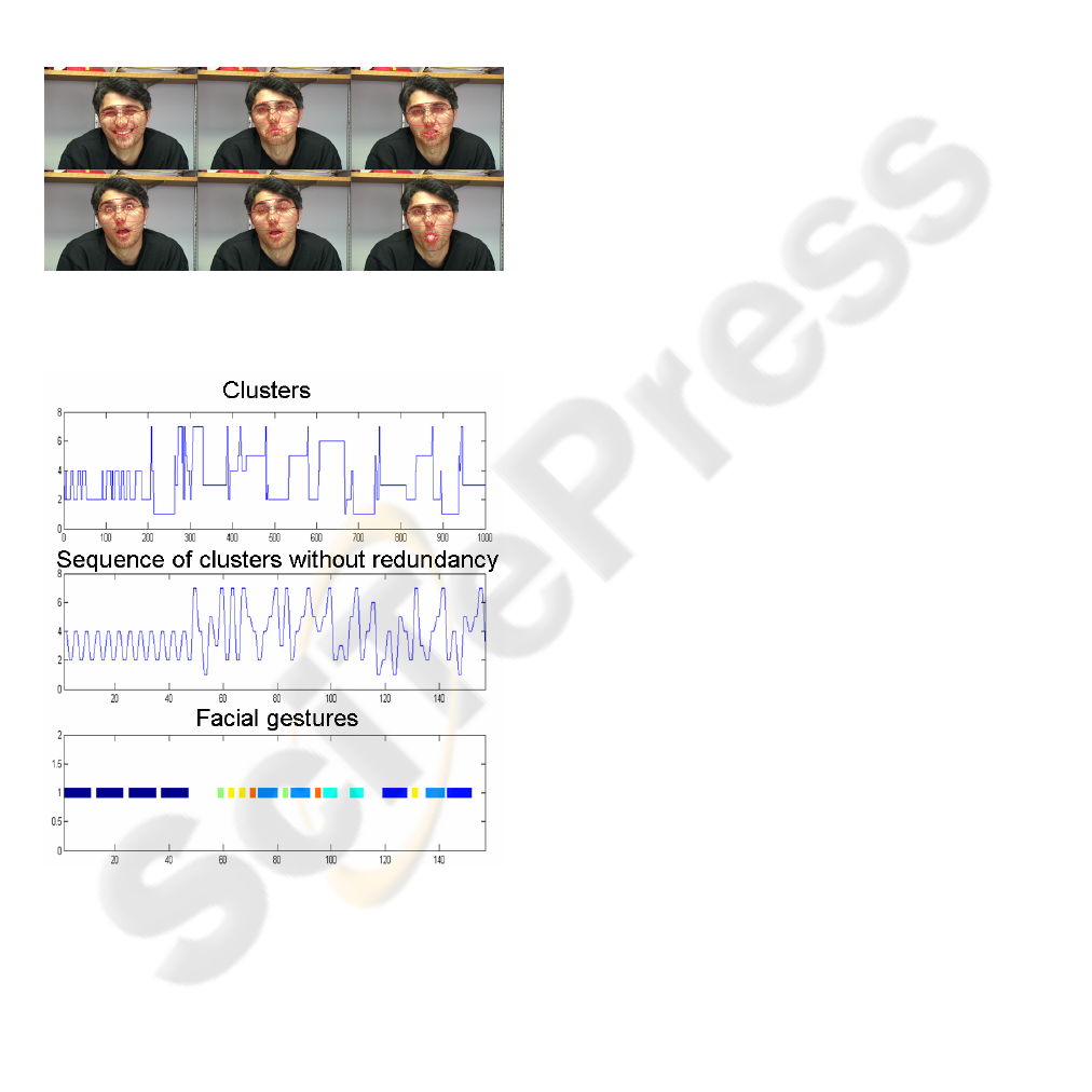
We have synthetically created three different shape
prototypes (fig. 5.b) and perturbed them with 50 ran-
dom affine transformations (fig. 5.a). After running
PaCA we can see the mean of the shape for each clus-
ter in the second row of fig. 5 is correctly recovered.
PaCA has correctly clustered the original shapes.
Figure 5: First row: superimposed perturbed shapes for
each cluster. Second row: superimposed aligned shapes.
Also original prototypes.
6.2 Expression Segmentation
In this experiment, we have recorded a video se-
quence where the face of the subject is naturally mak-
ing five different facial gestures (sad, taking out the
tongue, speaking, smiling, and neutral). We use AAM
VISAPP 2007 - International Conference on Computer Vision Theory and Applications
114

to track the sequence (see fig. 6). After the tracking
is done, we automatically detect the AU0 and remove
the temporal redundancy in the cluster sequence, re-
ducing the sequence to 20% its original length (see
fig. 7.a and 7.b). Later, the temporal segmentation
algorithm discovers the facial gestures shown in 7.c.
Observe that there are some time windows that are
not classified, this windows correspond to one time
or unusual facial gestures. We have visually checked
the correctness of our approach. The results in
video can be downloaded from www.cs.cmu.edu/ ∼
f torre/ExpressionSegmentation.avi.
Figure 6: AAM tracking across several frames.
Figure 7: a) Original sequence of clusters. b) Sequence
of clusters with just the transitions. c) Discovered facial
gestures.
REFERENCES
Adiv, G. (1985). Determining three-dimensional motion
and structure from optical flow generated by several
moving objects. IEEE transactions on Pattern Analy-
sis and Machine Intelligence, 7(4):384–401.
Cohn, J., Ambadar, Z., and Ekman, P. (2006). Observer-
based measurement of facial expression with the facial
action coding system.
de la Torre, F. and Kanade, T. (2006). Discriminative clus-
ter analysis. In International Conference on Machine
Learning.
Dhillon, I. S., Guan, Y., and Kulis, B. (2004). A unified
view of kernel k-means, spectral clustering and graph
partitioning. In UTCS Technical Report TR-04-25.
Ding, C. and He, X. (2004). K-means clustering via princi-
pal component analysis. In International Conference
on Machine Learning, volume 1.
Domke, J. and Aloimonos, Y. (2006). Deformation and
viewpoint invariant color histograms. In BMVC.
Fletcher, R. (1987). Practical methods of optimization. John
Wiley and Sons.
Hoey, J. (2001). Hierarchical unsupervised learning of fa-
cial expression categories. In Detection and Recog-
nition of Events in Video, 2001. Proceedings. IEEE
Workshop on s.
Jain, A. K. (1988). Algorithms For Clustering Data. Pren-
tice Hall.
Lucey, S., Matthews, I., Hu, C., Ambadar, Z., de la Torre,
F., and Cohn, J. (2006). AAM derived face represen-
tations for robust facial action recognition. In Proc.
International Conference on Automatic Face and Ges-
ture Recognition.
MacQueen, J. B. (1967). Some methods for classifica-
tion and analysis of multivariate observations. In 5-th
Berkeley Symposium on Mathematical Statistics and
Probability.Berkeley, University of California Press.,
pages 1:281–297.
Mase, K. and Pentland, A. (1990). Automatic lipreading by
computer. (J73-D-II(6)):796–803.
Matthews, I. and Baker, S. (2004). Active appearance mod-
els revisited. International Journal of Computer Vi-
sion, 60(2):135–164.
Shi, J. and Malik, J. (2000). Normalized cuts and image
segmentation. IEEE Transactions on Pattern Analysis
and Machine Intelligence, 22(8).
Zelnik-Manor, L. and Irani, M. (2004). Temporal factoriza-
tion vs. spatial factorization. In ECCV.
Zha, H., Ding, C., Gu, M., He, X., and Simon., H. (2001).
Spectral relaxation for k-means clustering. In Neural
Information Processing Systems, pages 1057–1064.
Zhao, W. and Chellappa, R. (2006). (Editors). Face
Processing: Advanced Modeling and Methods. El-
sevier.
SIMULTANEOUS REGISTRATION AND CLUSTERING FOR TEMPORAL SEGMENTATION OF FACIAL
GESTURES FROM VIDEO
115