DIFFERENNTIAL TECHNIQUE FOR MOTION COMPUTATION

USING COLOUR INFORMATION

T. Bouden and

(*)

N. Doghmane

NDT laboratory, Automatic Department, Engineering Faculty

BP°98 Ouled Aissa 18000 Jijel University, Algeria

(Temporary Trainee until August 2007: LIS/INPG Grenoble France)

(*)

Electronic Department, Campus Sidi Ammar 23000, Annaba University Algeria

Keywords: Differential techniques, optical flow, motion estimation and colour information.

Abstract: Optical flow computation is an important and challenging problem in the motion analysis of images

sequence. It is a difficult and computationally expensive task and is an ill-posed problem, which expresses

itself as the aperture problem. However, optical flow vectors or motion can be estimated by differential

techniques using regularization methods; in which additional constraints functions are introduced. In this

work we propose to improve differential methods for optical flow estimation by including colour

information as constraints functions in the optimization process using a simple matrix inversion. The

proposed technique has shown encouraging results.

1 INTRODUCTION

The recent developments in computer vision,

moving from static images analysis to video

sequences, have focused the research on the

understanding of motion analysis and representation.

A fundamental problem in processing sequences is

the computation of motion. Optical flow is a

convenient and useful way for image motion

representation and 3D interpretation. It often plays a

key role in varieties of motion estimation techniques

and has been used in many computer vision

applications. Optical flow may be used to perform

motion detection, autonomous navigation, scene

segmentation, surveillance system (motion can be an

important source for a surveillance system when

objects of interest can be detected and tracked using

the optical flow vector to define the future

trajectories), motion compensation for encoding

sequences and stereo disparity measurement (Barron

1994), (Beauchemin, 1995) and (Weickert, 2001).

Thus an optical flow algorithm is specified by three

elements (Barron, 1994):

* The spatiotemporal operators that are applied

to the image sequence to extract features and

improve the signal to noise ratio,

* How optical flow estimates are produced from

a gradient search of the extracted feature space, and

the form of regularization applied to the flow field

considering confidence measures if they exist.

Optical flow estimation and computation methods

can be classified into three main categorie:

differential approaches, block-matching approaches

and frequential approaches (Baron, 1994).

Despite more than two decades of research, the

proposed methods for optical flow estimation are

relatively inaccurate and non-robust. Many methods

for the estimation of optical flow have been

proposed (Horn and Shunck (Horn, 1981); Lucas

and Kanade (Lucas, 1981); Markandy and

Flinchbaugh (Markandy, 1990); Fleet and Jepson

(Baron, 1994) and (Beauchemin, 1995); Weber and

Malik (Weber, 1995); Polina and Golland (Polina,

1995); Tsai et al. (Tsai, 1999); Ming et al.

(Ming,2002); Zhang and Lu (Zhang, 2000); Bruno

and Pellerin (Bruno, 2003); Barron and Klette

(Barron, 2002), Arredondo and al. (

Arredondo ,

2004), Joachim Weickert and al. (Joachim, 2003),

(Thomax, 2004) and (André, 2005) and Volker

Willert and al (Volker, 2005) ) .

We present in this paper a differential approach

using colour components as constraints functions for

the optical flow computation. The rest of this paper

is organized as follows: section 2 describes the main

optical flow constraint equation. In section 3 we

describe how to use colour in the process of optical

531

Bouden T. and Doghmane N. (2007).

DIFFERENNTIAL TECHNIQUE FOR MOTION COMPUTATION USING COLOUR INFORMATION.

In Proceedings of the Second International Conference on Computer Vision Theory and Applications - IU/MTSV, pages 531-537

 SciTePress

flow estimation. In section 4, we present the method

for the minimization of the function including the

smoothing term based on colour information. Some

experimental results are presented in section 5 and at

the end, we address a conclusion.

2 OPTICAL FLOW CONSTRAINT

EQUATION

Optical flow is the apparent motion of brightness

patterns in the images sequence. It corresponds to

the motion field, but not always.

Optical flow techniques are based on the idea

that for most points in the image, neighbouring

points have approximately the same brightness.

Optical flow can be computed from a sequence by

using the (Horn, 1981) assumption, known as the

brightness constancy assumption, is represented by

the following equation:

Where:

, I

and I

are first partial derivatives of I

respectively with respect to x, y and t and u and v

are the optical flow components in the x and y

directions.

Equation (1) is called optical flow constraint

equation. It provides only the normal velocity

component. So we are only able to measure the

component of optical flow that is in the direction of

the intensity gradient (aperture problem) and the

system is undetermined. To overcome this problem,

it is necessary to add additional constraints.

Another problem is that are assuming that δt is very

small. The sampling error in the spatial domain also

leads to errors in the computation of the I

and I

3 USE COLOUR INFORMATION

AS CONSTRAINT

The brightness assumption implies that the (R, G, B)

components of each image remain unchanged during

the motion undergone within a small temporal

neighbourhood (Weber, 1995). Therefore, R, G and

B images can be used in a similar way as the

luminance function: they have to satisfy the optical

flow constraint equation. Markandey and

Flinchbaugh (Markandy, 1990) have proposed a

multispectral approach for optical flow computation.

Their two-sensors proposal is based on solving a

system of two linear equations having both optical

flow components as unknowns. The equations are

deduced from the standard optical flow constraint

(1). In their experiments, they use colour TV camera

data and a combination of infrared and visible

images. Finally, they use two channels to resolve the

ill-posed problem (Barron, 2002).

Golland and Bruckstein (Polina, 1995) follow

the same algebraic method. They compare a

straightforward 3-channels approach using RGB

data with two 2-channel methods, the first based on

normalized RGB values and the second based on a

special hue-saturation definition.

The standard optical flow constraint may be

applied to each one of the RGB quantities, providing

an over determined system of linear equations

(Barron, 2002):

Then the pseudo-inverse computation gives the

following solution for the system:

Where:

This assumes that the matrix (A

A) is non-singular.

By definition this matrix is singular if its

columns or lines are linearly dependent, which

means that the first order spatial derivatives of the

colour components (R, G, B) are dependent. Since

the sensitivity functions Dr(λ), Dg(λ) and Db(λ) of

the light detectors are linearly independent, the first

derivatives of the R, G, B functions will also be

independent for images sequence with colour

changing in two different directions. But if the

colour is a uniform distribution, the (R, G, B)

functions are linearly dependent or if the colours of

the considered region change in one direction only,

the gradient vectors of (R, G, B) are parallel so that

the spatial derivatives are dependent and the matrix

A) is singular. In addition to the estimates of the

image flow components at a certain pixel of the

image, we would like to get some measure of

confidence in the result at this pixel, which would

tell us to what extent we could trust our estimates. It

is common to use the so-called condition number of

the coefficient matrix of a system (A

A) as a

measure of confidence of this system (Polina, 1995).

To improve this problem, the idea is the use of two

independent functions for colour characterization so

that their gradient directions are not parallel. If the

xyt

Iu Iv I++=

(1)

xyt

Ru Rv R

Gu Gv G

Bu Bv B

⎧

⎪

⎨

⎪

⎩

(2)

(.)..

VAAAb

−

(3)

xy t

RR R

A G G b G and V

BB B

⎡⎤

−

⎡⎤

⎢⎥

==−=

⎢⎥

⎣⎦

⎢⎥

−

⎣⎦

(4)

VISAPP 2007 - International Conference on Computer Vision Theory and Applications

532

quantities used here are denoted f and ff. The colour

conservation assumption implies:

Here the solution is given by simple matrix

inversion:

The ideal case is obtained when the gradient

directions of the two chosen functions are normal.

One possible solution is the use of two different

colour systems: the normalized RGB system,

denoted rgb system and the HSV system (Barron,

2002), (Markandy, 1990) and (Polina, 1995).

It is clear that any pair of (r, g, b) forms a system of

two independent functions. If we are taking the r and

g components, the optical flow computation system

to be solved is given by equation (6), where:

Now we consider the HSV systems. H and S

describe a vector in polar form, representing the

angular and magnitude components respectively

(Robert, 2003).

The HSV space is computed in the following way:

The solution is given by equation (6), where:

4 PROPOSED METHOD

It was shown that a colour sequence could be

straightforwardly considered as a set of three

different sequences produced by three types of light

sensors with different sensitivity functions in

response to the same input sequence (Markandy,

1990) and (Polina, 1995). So we propose to use the

same formulation as those proposed by Horn and

Schunck for the luminance function and to apply it

to the three colour components.

In the first stage we have to minimize a function

error containing the three colour components for the

considered colour space, each component satisfying

the optical flow constraint equation without any

smoothness term, for the RGB space we have:

The problem will be posed as finding (u, v) optical

flow components minimising F. The solution was

given by using equation (6); Where:

The matrix A must be non-singular. The smallest

eigenvalue of A

A or the condition number of A

can be used to measure numerical stability, i.e. if the

smallest eigenvalue is below a threshold or the

condition number is above a threshold, then we set

the optical flow vector to be undefined at this image

location.

So, in the second stage we add a local (on a small

region around each pixel) smoothness term on the

magnitude of optical flow vector with a weight α.

The motion of any object between two successive

times (t

and t

+∂t where ∂tÆ0) is supposed to be

very small and it can be used as a small

displacement in any direction. So equation (9) with

the smoothness term will be:

(

)

(

)

()

xyt xyt

xyt

Min

F R .u R .v R ² G .u G .v G ²

B.u B.v B ²+

εε

⎧

= +++ ++

⎪

+++

⎨

⎪

=+++

⎩

(12)

Deriving F over u and v and solving the result

system. The same solution is found when adding the

smoothness term in the function F to minimize.

Deriving This solution is obtained by equation (6),

where :

We do not use iterative method to compute the

optical flow components here and the proposed

xyt

fu fv f

ff u ff v ff

++=

⎧

⎪

⎨

++=

⎪

⎩

(5)

.VAb

−

(6)

A b and V

gg v

−

== =

−

⎡⎤

⎢⎥

⎣⎦

(7)

(,,) (,,)

(,,)

(,,),

(,,) (,,)

2(,,),

(,,) (,,)

4(,,)

(,,) (,,)

(, , ),

Max R G B Min R G B

Max R G B

fRMaxRGB

Max R G B Min R G B

If G Max R G B

Max R G B Min R G B

fBMaxRGB

Max R G B Min R G B

VMaxRGB

−

⎧

−

⎪

−

⎪

−

=+ =

⎨

−

⎪

−

⎪

−

⎪

⎩

(8)

and

AbV

SSv

−

===

−

⎡⎤

⎢⎥

⎣⎦

(9)

(

)

(

)

()

xyt xyt

xyt

Mi n

FR.uR.vR²G.uG.vG²

B.u B.v B ²

εε

⎧

= +++ ++

⎪

+++

⎨

⎪

=++

⎪

⎩

(10)

222

;

222

RGBRRGGBB

x x xy xy xy

RR GG BB R G B

yxyxyyyy

RR GG BB

xxx

ttt

RR GG BB

yyy

ttt

++ + +

++ ++

=−

⎡

⎤

⎢

⎥

⎢

⎥

⎣

⎦

⎡⎤

⎢⎥

⎣⎦

(11)

2222

;

2222

RGB RRGGBB

x x xy xy xy

RR GG BB R G B

xy xy xy y y y

RR GG BB

xxx

ttt

RR GG BB

yyy

ttt

+++ + +

++ +++

=−

⎡

⎤

⎢

⎥

⎢

⎥

⎣

⎦

⎡⎤

⎢⎥

⎣⎦

(13

)

DIFFERENNTIAL TECHNIQUE FOR MOTION COMPUTATION USING COLOUR INFORMATION

533

method is only based on the function optimisation

and matrix inversion.

5 EXPERIMENTAL RESULTS

This section examines the quantitative performances

and the implementation of the proposed method.

5.1 Error Measurement

In order to quantify the accuracy of the estimated

range flow, the following errors measures are used.

Let the correct range flow be denoted as Vc and the

estimated flow as Ve. The relative error in the

velocity magnitude (

Barron et al., 2004), (Baron and

Klette, 2002), (

Volker et al., 2005):

[%]100.

−

(14)

We use the directional error as a second error

measure:

[]

arccos

VcVe

Vc Ve

⎛⎞

=°

⎜⎟

⎝⎠

(15)

This quantity gives the angle in 3D between

the correct velocity vector and the estimated vector

and thus describes how accurately the correct

direction has been recovered. We address this table,

to prove the efficiency of optical flow method for

studied sequences and for a precise confidence

measure (Barron, 2002), (

Arredondo, 2004),

(Joachim, 2003), (Thomax, 2004), (André, 2005)

and (Volker, 2005).

5.2 Implementations and Results

In the implementation of all studied methods, the

images of R, G and B, (r and g) and (H and S) are

obtained from the brightness function of images

sequence (R, G, B).

The first order derivatives of the sequence

functions are computed by using the (1/12) (-1, 8, 0,

-8, 1) kernel. We used a 5x5 neighbourhood, where

each line was a copy of the estimation kernel

mentioned above. For the computation of temporal

derivatives, a 3x3x2 spatiotemporal neighbourhood

was used.

In our case, we first computed the time taken by

any studied method addressed in Table 2, using

Matlab implementation on Toshiba PC Intel®

pentium®, Microprocessor 1.70GHz and 1Go of

RAM. We used the ball sequence with different

sizes and Barron and Klette synthetic panning

sequence in 2002.

The first synthetic sequence (figure 2), derived from

the original sequence (figure 1), contains ball

moving in the horizontal direction with 4

pixels/frame and in the vertical direction with 3

pixels/frames, with variable sizes. The second one is

generated by Barron and Klette (figure 7) where the

correct flow is known (Baron and Klette, 2002),

(

Volker et al., 2005).

Table 1: Time taken for computation by s CPU time.

In the second stage, we used the first synthetic

colour ball sequence with 64x64 size (figure 2) to

compare quantitatively the obtained results by each

studied method (figures 5 to 8). The results are

reported in table 2.

Table 2: Results Errors Comparison using synthetic colour

ball sequence with 64x64 size.

Proposed Method

AME :

Er±Std(Er)

AAE :

Ed±Std(Ed)

Using rgb space RGB 5.50%±2.44% 3.15°±1.39°

Using HSV space RGB 22.2%±25.45% 11.6°±12.14

Min. RGB space RGB 10.4%±11.41% 5.83°±6.13°

Min.(smooth.: α) RGB 6.16%±4.11% 3.52°±2.33°

In the last stage, we used the synthetic panning

sequence (figure 7) to compare quantitatively the

obtained results (figures 8 to 15). In table 4, we

added from the fourth line our results to the results

presented in (Baron and Klette, 2002), (

Volker et al.,

2005).

Table 3: Comparison between the results (Figures: 10 to

16) using synthetic panning sequence.

Method

AME :

Er±Std(Er)

AAE :

Ed±Std(Ed)

Horn-Schunck RGB 17.44%±17.77% 2.64°±4.08°

Goland-Bruckstein RGB 11.38%±17.36% 5.04°±11.80°

Baron-Klette RGB 16.14%±17.57% 0.16°

Using rgb space RGB 3.04%±0.72% 1.74°±0.40°

Using HSV space RGB 9.66%±19.14% 5.04°±8.63°

Min. RGB space RGB 6.06%±6.96% 3.43°±3.79°

Min. RGB space RGB

with smoothing term

3.52%±2.04% 2.01°±1.16°

Method 64x64 128x128 240X320 Panning

Using rgb 2.125 7.079 103.704 56.422

Using HSV 2.047 8.266 114.797 73.031

Using Min RGB 2.984 10.219 144.953 78.578

Using Smooth. α 3.062 10.625 146.719 83.781

VISAPP 2007 - International Conference on Computer Vision Theory and Applications

534

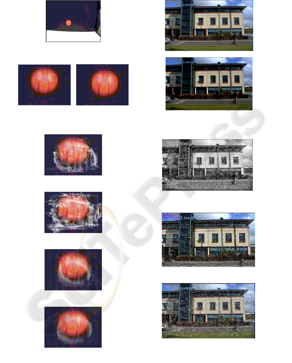
Figure 1: Original Image, of colour ball sequence with

240X320 size.

(a) (b)

Figure 2: (a) First image (b) Second image, of synthetic

colour ball sequence size 64X64.

Figure 3: Proposed method using rgb space.

Figure 4: Proposed method using HSV space.

Figure 5: Proposed method using RGB space.

Figure 6: Proposed method using RGB space with

smoothing term equal 3.

(a)

(b)

Figure 7: Images of Panning colour sequence (Real colour

sequence).

Figure 8: Horn-SchuncK flow for the Y component

(Y=0.299R+0.587G+0.114B) with α=3 and 100 iterations.

Figure 9: Golland-Bruckstein flow (RGB).

Figure 10: Baron-Klett flow (RGB).

DIFFERENNTIAL TECHNIQUE FOR MOTION COMPUTATION USING COLOUR INFORMATION

535

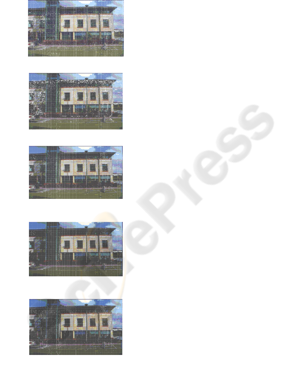
Figure 11: Proposed method using rgb space.

Figure 12: Proposed method using HSV space.

Figure 13: Proposed method using RGB space without

smoothing term.

Figure 14: Proposed method using RGB space with

smoothing term (α=100).

Figure 15: Proposed method using RGB space with

smoothing term (α=3).

6 CONCLUSION

When we propose a new method, its drawbacks

should also be discussed and compared with the

other methods in the same environment. It has

proved encouraging results.

Colour optical flow computed via the three

colour components seems better than grey value

optical flow. The proposed method using normalized

rgb colour space gives good results followed by that

using RGB space with smoothing term after that we

found the proposed method using RGB space

without smoothing term and finally that using the

HSV space. In our case we used a 100% density of

dense optical flow computation.

This proposed method requires the presence of

significant gradients of the functions it is based on.

If the gradient magnitude of these functions is small

enough (≈0), any gradient based method would fail

to give reliable results. This implies that all these

methods should not be used when a scene contains

objects with uniform colour.

The proposed method used the least squares

techniques to minimize the combination of optical

flow colour constraint equation using the matrix

inversion to compute the dense flow optic. We have

used the brightness constancy assumption, the colour

information as constraint function and the same

smoothness function as that proposed by Horn and

Shunck.

We can extend the proposed smoothness function

with other forms (as the combination of the local and

global constraints) and we can use a bidirectional

multigrid method for variational optical flow

computation to resolve the real-time computation

problem and the solving of the linear system of

equations that results from the discretisation of the

Euler-Lagrange equations.

We plan to investigate all these to find a robust

and sufficiently method for optical flow computation

for any given sequences in some specific

applications.

REFERENCES

Arredondo M. A., Lebart K. and Lane D., 2004. Optical

flow using texture. In Pattern Recognition letters in

Elsevier computer science, Letters25.

Barron J. L., Fleet D. J., Beauchemin S. S. and Burkitt T.

A., 1994. Performance of optical flow techniques. In

IJCV 12 (1).

VISAPP 2007 - International Conference on Computer Vision Theory and Applications

536

Barron J. L. and Klette R., 2002. Quantitative colour

optical flow. In Proc. Int. Conf. on Pattern

Recognition.

Beauchemin S. S. and Barron J. L., 1995. The

Computation of Optical Flow. In ACM Computing

Survey, 27(3).

Bruno E. and Pellerin, D., 2000. Robust motion estimation

using spatial gabor filters. In X European Conf. Signal

Process.

Horn B. K. P. and Schunck, B. G., 1981. Determining

optical flow. In A.I.17.

Lucas B. D. and Kanade T., 1981. An iterative image

registration technique with an application to stereo

vision. In 7th Int. Joint Conf. on Artificial Intelligence.

Markandy V. and Flinchbaugh B. E., 1990. Multispectral

constraints for optical flow computation. In Proc. 3rd

ICCV, Osaka, Japan.

Ming, Y., Haralick, R. M. and Shapiro, L. G., 2002.

Estimating optical flow using a global matching

formulation and graduated optimization. In Proc. Int.

Conf. on Image Process.

Polina Golland, 1995. Use of colour for optical flow

estimation. In master of science in computer science,

Israel institute of Technologies, Iyar 5755 Haifa.

Tsai C. J., Galatsanos N. P. and Katsaggelos A. K., 1999.

Optical flow estimation from noisy data using

differential techniques. In Proc. IEEE Int. Conf. on

Acoustics, Speech, and Signal Process., vol. 6.

Weickert J. and Schnörr C., 2001. Variational optic flow

computation with a spatio-temporal smoothness

constraint. In Journal of Mathematical Imaging and

Vision.

Weber J., Malik J., 1995. Robust computation of optical-

flow in a multiscale differential framework. In IJCV

14 (1).

Zhang D. and Lu G., 2000. An edge and colour oriented

optical flow estimation using block matching. In:

Proc.5th Int. Conf. on Signal Process.

Robert J. A and Brian C. Lovell, 2003. Color Optical

Flow. In Lovell, Brian C. and Maeder, Anthony J, Eds.

Proceedings Workshop on Digital Image Computing,

pages 135-139, Brisbane.

Joachim W., André B and Christoph S., 2003.

Lukas/Kanade Meets Horn/Schunck: Combining

Local and Global Optic Flow Methods. PrePrint N°82.

In Fachrichtung 6.1- Mathematik Universität des

Saarlandes.

Thomax B., André B., Nils P. and Joachim W., 2004. High

Accuracy Optical Flow Estimation Based on a theory

for warping. In Proc., 8

European Conf. on

Computer Vision, Springer LNCS 3024, T. Pajdla and

J. Matas (Eds.), vol.4, PP:25-36, Prague, Czech

Republic.

André B., Joachim W., Christian F., Timo K. and

Christoph S., 2005. Variational optical flow

computation in real time. In IEEE Transactions on

Image Processing. Volume 14, Num.1.

Volker W., Julian E., Sebastian C. and Edgar K.; 2005.

Probabilistic colour optical flow. In W. Kropatsch, R.

Sablatnig, and Hanbury (Eds): DAGM 2005, LNCS

3663; PP:9-16; Springer-Verlag Berlin Heidelberg.

DIFFERENNTIAL TECHNIQUE FOR MOTION COMPUTATION USING COLOUR INFORMATION

537