
IMPROVEMENTS IN SPEAKER DIARIZATION SYSTEM
Rong Fu and Ian D. Benest
Department of Computer Science, the University of York, YO10 5DD, York, UK
Keywords:
Speaker Diarization, Model Complexity Selection, Universal Background Model.
Abstract:
This paper describes an automatic speaker diarization system for natural, multi-speaker meeting conversations
using one central microphone. It is based on the ICSI-SRI Fall 2004 diarization system (Wooters et al., 2004),
but it has a number of significant modifications. The new system is robust to different acoustic environments
- it requires neither pre-training models nor development sets to initialize the parameters. It determines the
model complexity automatically. It adapts the segment model from a Universal Background Model (UBM),
and uses the cross-likelihood ratio (CLR) instead of the Bayesian Information Criterion (BIC) for merging.
Finally it uses an intra-cluster/inter-cluster ratio as the stopping criterion. Altogether this reduces the speaker
diarization error rate from 25.36% to 21.37% compared to the baseline system (Wooters et al., 2004).
1 INTRODUCTION
For the purposes of this paper, speaker diarization is
the process by which an audio recording of a meeting
is indexed according to the speakers who made oral
contributions. The NIST Rich Transcription Eval-
uations (NIST, 2004) refers to this as “who spoke
when”. Research in speaker diarization currently fo-
cuses on three main areas. First, through its indexing
and modelling, diarization enables audio databases
to be searched for particular individuals. Second,
the provision of diarization improves the success rate
of automatic speech recognisers by enabling them
to adapt to different speakers. The third application
is in the provision of more structured transcripts of
recorded meetings, news broadcasts and telephone
conversations (Tranter and Reynolds, 2006). It is the
first area on which this paper focuses. The process
reported here is performed without the knowledge of,
for example, the number of speakers involved, their
gender, and the positions of extraneous noises such as
laughter, coughing, paper shuffling and so on. While
meetings can be recorded using either a single cen-
tral microphone or multiple-microphones (where each
person has their own microphone) (Jin et al., 2004),
this work concentrates on single-microphone record-
ings of meetings between a number of individuals. Of
course the system needs to be robust with regard to the
acoustic environment - implying that there should be
no pre-training of the acoustic models, and the tuning
of parameters should be automatic.
The system described in this paper is based on
the ICSI-SRI Fall 2004 diarization system (Wooters
et al., 2004). This was selected because it adopts
the single microphone speaker diarization task, and
performs acoustic modelling using only the audio file
itself. In contrast with their system (Wooters et al.,
2004), this new one adopts an alternative approach to
determining the model complexity parameters auto-
matically, using the cross log-likelihood ratio rather
than the Bayesian Information Criterion (BIC) as the
merging rule; in addition it uses the intra-cluster/inter-
cluster ratio as the criterion for identifying the number
of speakers.
The paper is structured as follows. Section 2 de-
scribes the basic diarization system adopted by Woot-
ers et al.(2004), which is taken to be the baseline for
comparison. In section 3 the techniques used to im-
prove on the basic system are described. The experi-
mental arrangement and results are presented in sec-
tion 4 and conclusions are offered in section 5.
317
Fu R. and D. Benest I. (2007).
IMPROVEMENTS IN SPEAKER DIARIZATION SYSTEM.
In Proceedings of the Second International Conference on Signal Processing and Multimedia Applications, pages 313-319
DOI: 10.5220/0002140703130319
Copyright
c
SciTePress

2 THE BASELINE DIARIZATION
SYSTEM
In the ICSI-SRI Fall 2004 diarization system a guess
is made as to the number of individual speakers (K);
that guess must be much greater than the number of
actual speakers. The audio file is divided up into
60 millisecond windows with each window overlap-
ping the previous one by 20 milliseconds. For each
window, nineteen mel-frequency cepstral coefficients
(MFCC) are extracted as acoustic feature vectors for
that window. These feature vectors are assigned se-
quentially to the K speakers; this grouping of fea-
ture vectors is called a segment (and there are K seg-
ments). Wooters et al. (2004) report that this speaker
change detection initialization method is as effective
as those based on distance measures (Barras et al.,
2004) or BIC (Zhou and Hansen, 2000).
A K state Hidden Markov Model (HMM) is cre-
ated where, of course, each of its states acoustically
models a single potential speaker. Gaussian Mixture
Models (GMM) are established to initialize the states
of the HMM. The Viterbi decoding algorithm is used
to re-assign feature vectors to other states and the
GMM is thus updated. Several sub-states are linked
to each K state and these share the state’s probability
density function (pdf). Upon entering a state, the fea-
ture vectors cannot change to another state unless they
have travelled through all the sub-states one-by-one.
This imposes a minimum number of features (equiva-
lent to more than 0.9 seconds), which are assigned to
a state each time. This iteratively refines the segment
boundary assigned to each state. This approach was
first reported by Ajmera et al.(2002).
Wooters et al. (2004) advise that an agglomerative
clustering technique with BIC merging and stopping
criteria (Ajmera and Lapidot, 2002) always gives the
best performance for clustering segments. Bayesian
Information Criterion (BIC) (Schwarz, 1978) is a
model selection criterion which prefers those models
that have large log-likelihood values, but penalizes it
with model complexity (the number of parameters in
the model) (Schwarz, 1978). For a pair of segments x
and y which are assigned to different states, their BIC
merging score is computed according to Eq.1.
BIC
score
= L
z
− (L
x
+ L
y
) −1/2α(P
z
log(n
z
) − P
x
log(n
x
) − P
y
log(n
y
)), (1)
where L
z
is the log-likelihood function for the merg-
ing model, P is the number of parameters used in the
model and n is the number of features in the segment.
The pair of states whose segments have the highest
BIC score will be merged, and the state model re-
trained. The merging process continues until there are
run speech/non-speech detection
extract feature vectors
initialize K-state HMM model
initialize
GMM for
each state
build the UBM based
on the audio file itself
and set the model
complexity
automatically
use MAP-adaptation to
initialize the GMM
model for each state
run Viterbi decoding to reassign the features
adapt the GMM from the UMB
for each state
compute the CLR for all pairs of
states
use normalized cuts to merge the
states
compute the
intra-cluster/inter-cluster ratio
if K = 1 if K > 1
output the result
with minimum
intra-cluster/inter-cluster ratio
update the GMM for each state
select the pair of segments with
largest BIC score
merge them if
BIC score > 0
stop if BIC
score < 0
output result
original ICSI
original
ICSI
new
system
new system
Figure 1: The original ICSI method compared with the new
system.
no pairs of states whose BIC score is larger than zero;
the clustering then stops. In the ICSI-SRI diarization
system, the number of parameters used in the merging
model is set to be equal to the sum of the number of
parameters used in each model, so the α parameter is
not required. The states that remain in the HMM are
potential speakers; the segments are thus indexed and
categorised. Ajmera and Wooters (2003) have created
an alternative algorithm which integrates the segmen-
tation and clustering together.
Sinha and Tranter (2005) and Barras et al. (2006)
have included a post-processing step in the speaker
diarization system in order to improve the perfor-
mance. This involves a Universal Background Model
(UBM), which is pre-trained either with other audio
files or with the data itself, and a Maximum a Pos-
teriori (MAP) mean-adaptation (Barras and Gauvain,
2003) is then applied to each cluster from the UBM
to give the state model. The Cross-Likelihood Ratio
(CLR) (Sinha et al., 2005) instead of BIC is applied
as the merging criterion.
Figure 1 illustrates and contrasts the original ICSI-
SRI system with that described by the authors.
SIGMAP 2007 - International Conference on Signal Processing and Multimedia Applications
318

3 THE NEW APPROACH
3.1 Model Complexity Selection
Model complexity is defined as the number of param-
eters within the model. For the Gaussian Mixture
Model with a fixed dimension and covariance type
(diagonal or full), the parameter which determines the
model complexity is the number of components in the
mixture model. In speaker diarization systems, there
are two steps which are influenced by the model com-
plexity; which pair of segments are to be merged, and
how should the model for a new segment be estab-
lished. A GMM with a small number of components
is too general and tends to over-merge the segments,
while a GMM with a large number of components is
too specific and tends to under-merge the segments.
Usually GMMs are trained by the EM algorithm and
unfortunately this is sensitive to the initialization en-
vironment. As a result an inappropriate estimate of
the number of components reduces the accuracy of
the model.
Anguera et al. (2005), and Wooters et al. (2004)
pre-determine this complexity with a fixed value; so
the model complexity cannot be changed according
to segment length and model similarity. The problem
is that a small segment with high complexity loses its
generalization. Anguera et al. (2006) automatically
determined the number of components depending on
the length of the segments. However, there was still
a need for a parameter that was adjusted by external
training sets. A problem also arose from the merging
process: the model of a populated segment doubles its
size after merging two segments of the same length,
ignoring both the similarity between the two segments
and their common speaker characteristics. The prob-
lem becomes more serious when UBM is introduced
to derive the segment models - as discussed in section
3.2.
The approach developed by Figueiredo and Jain
(2002), which overcomes the sensitivity limitation of
the EM algorithm, was adopted in the new system, but
with a modified stopping criterion. It automatically
determines the model complexity, and gives a model
that better fits the data.
Consider a finite data set X = {x
1
,x
2
,...x
n
} ⊂ ℜ
d
,
and an M-component GMM finite mixture distribu-
tion of dataset X, its pdf can be written as:
p(x|θ) =
M
∑
m=1
π
m
p(x|µ
m
,σ
m
). (2)
where
∑
M
m=1
π
m
= 1 and π
m
≤ 1,m = 1,··· ,M. π
m
is the mixing parameter of the mixture model, and µ
m
and σ
m
are the mean and covariance parameters of the
Gaussian component m. Then logp(X|θ) is defined
as:
logp(X|θ) =
n
∑
i=1
log
M
∑
m=1
π
m
p(x
(i)
|µ
m
,σ
m
). (3)
θ = {π,µ,σ} (4)
Usually an EM algorithm is applied to obtain the max-
imum likelihood (ML) estimate
ˆ
θ
ML
:
ˆ
θ
ML
= argmax
θ
{logp(X|θ)} (5)
The EM algorithm (McLachlan and Krishnan, 1997)
runs iteratively with an E-step followed by an M-step.
The E-step computes the conditional expectation of
the complete log-likelihood, given the dataset and
current estimate of all parameters - the so-called Q-
function. The M-step updates the estimate of θ in or-
der for it to maximize the Q-function (McLachlan and
Krishnan, 1997). The EM algorithm will monotoni-
cally increase the logp(x|θ) value until it reaches one
of the local maxima. Using the EM algorithm to train
the GMM model, label variables Z = {z
1
,··· ,z
n
} are
introduced so as to indicate which component pro-
duces which sample. The conditional expectations of
z
i
m
, where z
i
m
is the label which shows whether data
x
i
is produced by component m at iteration t, is given
by:
o
t
m
(x
i
) = E[z
t
m
|x
i
,
ˆ
θ
t
] =
ˆ
π
t
m
p(x
i
|
ˆ
θ
t
m
)
∑
M
j=1
ˆ
π
t
m
p(x
i
|
ˆ
θ
t
m
)
(6)
and π
t+1
m
will be updated thus:
π
t
m
=
n
∑
i=1
o
t
m
(x
i
)/n; (7)
o
i
m
is the posteriori probability of Z
i
m
, given the ob-
servation x
i
. Since the EM algorithm theoretically
searches the local maxima, its result is sensitive to
its initialization values. The results can always be
adjusted to get a better global maximum by split-
ting or merging the components (Ueda et al., 2000).
Figueiredo and Jain (2002) developed an algorithm
that successfully determines the number of compo-
nents used in building the GMM, and, at the same
time, optimizes the distribution of components. It
seamlessly integrates the Minimum Message Length
(MML) criterion into the EM algorithm. MML, like
BIC, is a model selection criterion. It is based on
information coding theory and was first developed
by (Wallace and Dowe, 1987). It prefers the model
which minimizes the right-hand side of Eq.8:
Length(
ˆ
θ,X) = −logp(
ˆ
θ) − logp(X|
ˆ
θ)
+
1
2
log|I(
ˆ
θ)| + p/2(1+ log(1/12)), (8)
IMPROVEMENTS IN SPEAKER DIARIZATION SYSTEM
319

where p is the number of parameters in the model.
Figueiredo and Jain (2002) assumed an independence
between the mixing parameter π and the compo-
nent parameter
ˆ
θ(m), and expresses a standard non-
informative Jeffreys’s prior for π, and
ˆ
θ,
p(
ˆ
θ
m
) ∝
q
|I
(1)
(
ˆ
θ
m
)|; (9)
p(π
1
,··· ,π
M
) =
p
|H| = (π
1
π2· ··π
M
)
−1/2
; (10)
and approximates |I(θ)| to |I
c
(θ)|, the complete-data
Fisher information matrix, which is described by
Eq.11:
I
c
(θ) = n∗ block− diag{π
1
I
1
(
ˆ
θ
1
),··· ,π
M
I
1
(
ˆ
θ
M
),H},
(11)
where I
1
(θ
m
) is the Fisher matrix for a single observa-
tion produced by the mth component, with |H| defined
in Eq.10. Then Eq.8 can be rewritten as:
Length(
ˆ
θ,X) =
N
2
M
∑
m=1
log(nπ
m
) +
p
2
(1+ log
1
12
)
+
p
2
log(n),
(12)
where p in Eq.8 is equal to NM + M, where N is the
number of parameters in each component. When the
π
m
of a component m is equal to 0, the component
will no longer contribute to the model, so then M is
the number of components whose mixing parameter
π
m
is larger than 0. Eq.12 is the criterion provided by
Figueiredo and Jain (2002), which can be integrated
into the EM algorithm in a closed form. In Eq.12,
the term
N
2
∑
M
m=1
log(nπ
m
) containing the variable π
is combined with Eq.5; then this is maximized:
∂(logp(X|
ˆ
θ))
∂π
m
+ λ(
M
∑
m=1
π
m
− 1) +
N
2
M
∑
m=1
log(nπ
m
)) = 0,
(13)
Instead of Eq.7, Eq.14 is calculated as the update
value for π
m
:
π
t
m
=
1
n− MN/2
(
n
∑
i=1
max(o
t
m
(x
i
) − N/2,0)) (14)
where o
t
m
(x
i
) is defined as in Eq.6.
By initializing the model complexity to a large
value M, this algorithm will reduce the complexity
value to M
n
by removing the components that have
insufficient evidence to support them. But there may
be an additional decrease in Eq.12 caused by a de-
crease in M
n
. So the algorithm needs to compute
the criterion value for each possible M
n
in order to
get the best result. This is computationally expensive
when the number of components is large. An alter-
native stopping criterion is the local Kullback-Leibler
divergence criterion in which those components with
the lowest local Kullback-Leibler divergence are re-
moved and the model retrained until the value of the
right side of Eq.12 no longer decreases. The local
Kullback-Leibler divergence criterion of component
m is described by Eq.15:
J
merge
(m|
ˆ
θ) =
f
m
(x|
ˆ
θ)log
f
m
(x|
ˆ
θ)
f
′
m
(x|
ˆ
θ)
dx, (15)
where f
m
is the current density function g, and f
′
m
is
the density function g
′
, whose component m has been
removed, all weighted by the posteriori function of m:
f
m
(x|
ˆ
θ) = g(x
i
)p(m|x
i
,
ˆ
θ); (16)
f
′
m
(x|
ˆ
θ) = g
′
(x
i
)p
′
(m|x
i
,
ˆ
θ); (17)
3.2 UBM and MAP Adaptation
Sometimes the segment is short and may be disturbed
by the acoustic environment so that the model on
which it is based is not sufficient to represent the
speaker characteristics. Then the Universal Back-
ground Model (UBM) is introduced to derive the seg-
ment models as referred to earlier in section 2.
UBM is always pre-trained from other speech cor-
pora. The audio file itself can be used to train the
UBM, or a combination of corpora and the speech file
may be used (Sinha et al., 2005) (Barras et al., 2006).
The authors adopted the audio file itself to build the
UBM and used the technique described in the last sec-
tion to develop the background model. A mean-only
MAP adaptation is always used to build the segment
model from the UBM. It updates the components’
means in the segment model by adapting them from
the UBM gradually. However, sometimes the seg-
ments produced by the system are very short and not
sufficient to cover the space modelled by the UBM.
As a result there may be some loss of segment char-
acteristics - hence the reason why this technique is
always applied as a secondary stage.
The authors’ system adjusts the weight parameter
in the UBM and removes those components for which
there is insufficient evidence (according to Eq.14) for
their retention. This step is used at the beginning
of the process, so determining the complexity of the
UBM model is important. The adapted weight esti-
mator is described by Eq.18
ˆ
π
m
=
max(
∑
n
i=1
p(m|x
i
) − N/2,0)
∑
k
m=1
max(
∑
n
i=1
p(m|x
i
) − N/2,0)
, (18)
SIGMAP 2007 - International Conference on Signal Processing and Multimedia Applications
320

where N is the number of parameters in each compo-
nent, and p(m|x
i
) is the posteriori probability of com-
ponent m given x
i
. Usually the mean-MAP adaptation
is then performed (Barras and Gauvain, 2003):
ˆµ
m
=
1
2
µ
i
+
1
2
(
∑
n
i=1
p(m|x
i
)x
i
)
1
2
+
1
2
∑
n
i=1
p(m|x
i
)
, (19)
This adaptation is performed for two iterations.
3.3 Cross-likelihood Ratio
CLR is used in place of BIC as the merging measure
adopted in most post-processing stages. Between any
two given segments s
i
and s
j
, CLR is defined by:
CLR(s
i
,s
j
) = log(
L(x
i
|θ
j
)L(x
j
|θ
i
)
L(x
i
|θ
ubm
)L(x
j
|θ
ubm
)
), (20)
where L(x
i
|θ
j
) is the average likelihood of the acous-
tic feature being in segment i given the model j, thus
removing the influence of the length of the segments
(Sinha et al., 2005). The CLR values are computed
for each pair of segments to form the CLR matrix.
3.4 Intra-cluster/Inter-cluster Ratio
Using BIC to merge and judge the stopping of the
speaker diarization task is, computationally, a local
solution. It considers those pairs of segments that
have the highest BIC score, without a global view of
the overall similarity between segments. The authors
found that it always under-estimated the number of
speakers appearing in the audio file. Futhermore in
the new system, CLR is applied as the merging cri-
terion instead of BIC; and BIC is no longer the natu-
ally stopping criterion. So in place of BIC, an intra-
cluster/inter-cluster ratio was used as the stopping cri-
terion. Intra-cluster/inter-cluster ratio compares the
way in which a state model represents its features,
with how the models of other states represent those
features; in so doing, it takes a global view of all the
states. Assuming that there are k clusters left in the
HMM, the intra-cluster/inter-cluster ratio is computed
by Eq.21:
intra− cluster
inter − cluster
=
k
∑
i=1
CLR(s
i
,s
i
)
∑
j, j6=i
CLR(s
i
,s
j
)
. (21)
The new system iteratively merges the segments un-
til there is only one segment left. Then the speaker
diarization solution is the cluster solution with mini-
mum intra-cluster/inter-cluster ratio.
4 EXPERIMENT
4.1 Data
The experiments reported in this paper used 36
recorded meetings as evaluation data, 18 from the
Interactive Systems Laboratories (ISL) part A meet-
ing corpus (ISL, 2004) and 18 from the International
Computer Science Institute (ICSI) meeting speech
corpus (ICSI, 2004). The average meeting length
was around 40 minutes, and the number of speakers
present in the meetings varied from 3 to 9. In the
meeting audio files, speaker changes are frequent, and
most have a short duration. Many exchanges overlap
with each other, hindering the speaker diarization.
4.2 Speaker Diarization Error
The baseline metric of performance is the diarization
error rate (DER), which is defined by NIST (2004).
It is obtained by comparing the results of diarization,
with a manually labelled transcript. The DER process
recognises three error types: the missed rate (speech
in the transcript that is not found by the system un-
der test), false alarm rate (speech found by the system
that is not in the transcript) and speaker error rate (the
sound is assigned to the wrong speaker). These are
computed by matching the speakers assigned by the
system to those in the transcript, using a one-to-one
mapping that maximises the total overlap between the
transcript and system speakers (as explained in (NIST,
2004)).
The main application of the new system is to index
and cluster the audio files. Usually the type of non-
speech appearing in the meeting audio files is silence
and noise. The false alarm rate does not influence the
indexing and clustering, nor does the missed speech
fragments as these last for less than 0.3 seconds. So an
energy based speech/non-speech detection is enough.
Since DER is a time-weighted evaluation measure, it
is primarily driven by dominant speakers. To reduce
the DER error rate, it is more important to find the
main speakers completely and correctly rather than
accurately find the speakers who do not speak very
often. Therefore when there is a dominant speaker
in the audio file, the DER measure fails to evaluate
how well the sytem finds other speakers. So segment
purity (SEGP) and speaker weighted speaker purity
(SPKP) are also introduced to evaluate the system.
Segment purity is a measure of how much speech in a
segment belongs to the correct speaker. Speaker pu-
rity measures how much speech is assigned correctly
to a speaker, weighted by the number of speakers.
IMPROVEMENTS IN SPEAKER DIARIZATION SYSTEM
321
In the new system, the 19
th
order MFCC was used
as acoustic feature vectors, extracted from 30 mil-
lisecond analysis windows each overlapping the pre-
vious one by 20 milliseconds. The initial guess at the
number of speakers was 40, and the minimum length
constraint was 0.9 seconds.
4.3 Conversation Overlap
Since there are many oral exchanges that overlap each
other in the audio files, it is possible that these re-
duce system performance, and this was investigated
in three experiments. First, the overlapping parts
were removed from the audio file and the diarization
system applied. Second, the overlapping parts were
included in the speaker diarization process, but ig-
nored in the evaluation process. Third, the overlap-
ping parts were included in the speaker diarization
process and, during evaluation, those parts were as-
signed to a speaker. Perhaps surprisingly, both the
second and the third experiments gave better results
than the first experiment. It seems that the overlap-
ping parts actually help to build the speaker models
and thus do not degrade the recognition rate. How-
ever, sometimes the overlapped parts are regarded as
new speakers, making the number of people detected
more than those actually present. The third approach
gives the best result because the overlapping speech
assigned to either of the speakers is thought to be cor-
rect.
4.4 Model Complexity
Three different methods for determining the model
complexity were investigated: first, fixing the num-
ber of Gaussians in the GMM; second, automatically
determining the value for model complexity depend-
ing on the segment length - the method adopted by
Anguera et al. (2006); and third, doing the same as
number two, but using the approach introduced for
the new system. A diagonal GMM was used and over-
lapped speech was ignored during the evaluation. All
three were integrated into the original ICSI system,
and their results are compared in Table 1. The ap-
proach used in the new system performed well when
the segments were short. However, it is computation-
ally expensive to find the number of components in
a long segment, and only gives slightly better results.
Since the approach is robust to the initialization envi-
ronment, its results are stable.
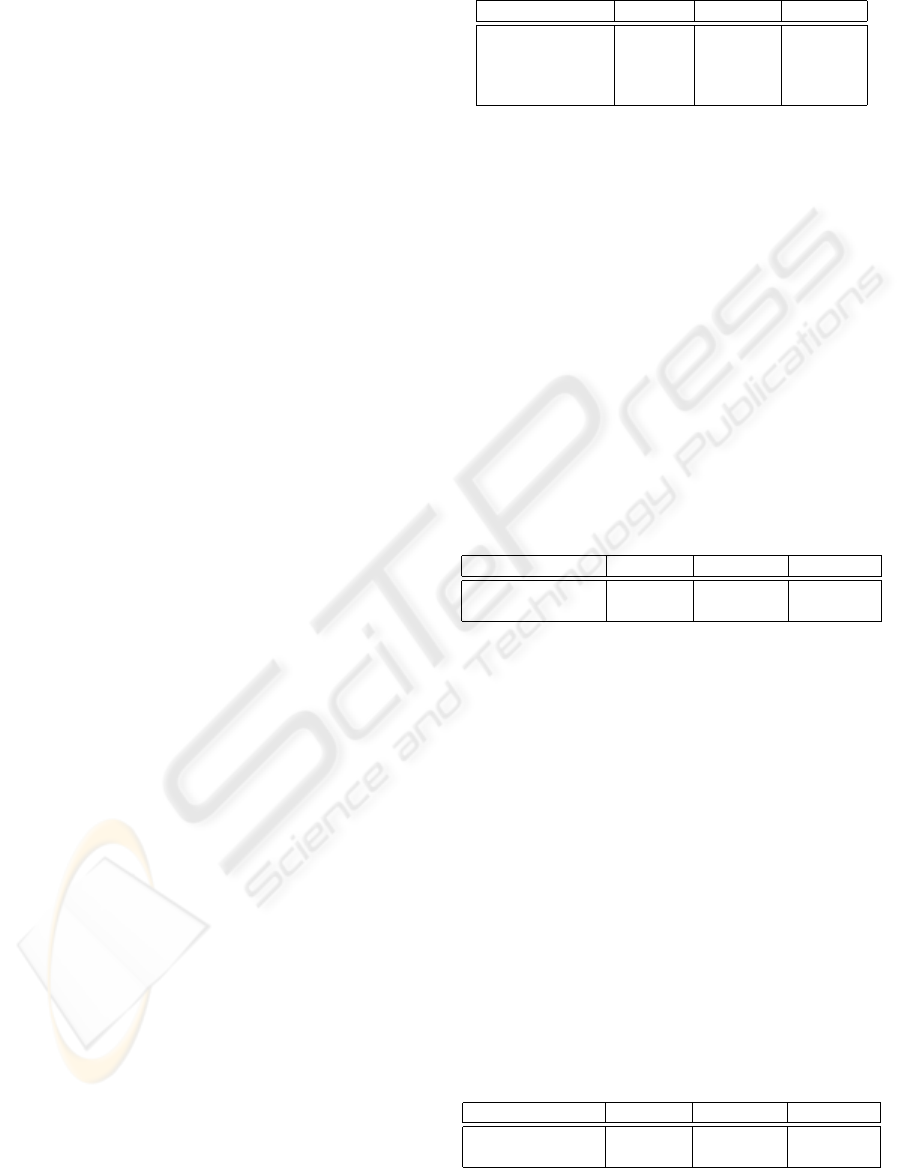
Table 1: Model-Complexity-Determining Methods.
method DER(%) SEGP(%) SPKP(%)
5 Gaussian/GMM 25.36 26.83 32.76
8 Gaussian/GMM 26.35 28.76 34.76
Anguera et al 22.25 22.76 28.76
authors’ approach 22.74 24.76 30.76
4.5 Applying the UBM
This part provides the biggest improvement. The new
EM approach used to train the GMM can automati-
cally remove the inefficient components, helping to
adapt the segment model from the UBM, especially
for short segments. Table 2 shows the difference be-
tween the segment model adapted from the UBM,
and that obtained from the ICSI system. Again, the
overlapped speech was ignored during the evaluation.
The UBM was built from the audio data itself and its
model complexity was automatically determined. The
segment models were then adapted from the UBM by
weight and mean-MAP. BIC was retained for deter-
mining the merging and stopping criteria.
Table 2: Effect of UBM-MAP Adaptation.
method DER(%) SEGP(%) SPKP(%)
UBM-MAP 19.74 21.85 28.36
Non UBM-MAP 25.36 26.83 32.76
4.6 Merging and Stopping Criteria
Finally, CLR and intra-cluster/inter-cluster ratio were
used instead of BIC for the merging and stopping
criteria. CLR seems to work well with the UBM
adapted segment model. It considers the similar-
ity between the segments and their similarity with
the UBM. The intra-cluster/inter-cluster stopping cri-
terion still under-estimates the number of speakers;
this may happen when there is a dominant speaker
at the meeting or the utterances from some speakers
are short. This stopping criterion almost correctly de-
tected the number of speakers, but the overall speaker
error rate was degraded. As shown in Table 3, the new
system reduces the error rate from 25.36% to 21.37%,
an improvement of about 19%. These results are ob-
Table 3: Overall Performance (without the overlap speech).
method DER(%) SEGP(%) SPKP(%)
Baseline System 25.36 26.83 32.76
New System 21.37 22.56 27.40
tained when the overlapped parts were ignored during
SIGMAP 2007 - International Conference on Signal Processing and Multimedia Applications
322

the evaluation. The best results, for both the baseline
system and the new one, were achieved when the re-
sults were evaluated using the approach that included
the overlapped parts, as shown in Table 4.
Table 4: Overall Performance (including the overlap).
method DER(%) SEGP(%) SPKP(%)
Baseline System 21.76 23.23 29.76
New System 17.21 18.56 26.40
In comparison with the ICSI system the diariza-
tion error rate was reduced from 21.76% to 17.21%.
5 CONCLUSION
This paper has described a new speaker diarization
system for natural, multi-speaker meeting conversa-
tions based on a single microphone. The system re-
quires no prior training, and the experiments showed
that the performance achieved 21.37% speaker di-
arization error rate. It is expected that different
speech/non-speech detection techniques and further
purity tests will improve the performance of the sys-
tem.
REFERENCES
Ajmera, J. and Lapidot, I. (2002). Improved unknown-
multiple speaker clustering using hmm. In IDIAP RR.
pp.02–23.
Barras, C. and Gauvain, J. L. (2003). Feature and score
normalization for speaker verification of cellular data.
In ICASSP Proc.
Barras, C., Zhu, X., Meignier, S., and Gauvain, J. L. (2004).
Improving speaker diarization. In Fall 2004 Rich tran-
scription Workshop (RT-04) Proc.
Barras, C., Zhu, X., Meignier, S., and Gauvain, J. L. (2006).
Multistage speaker diarization of broadcast news. In
IEEE Trans. SL Proc. pp.1505–1512.
ICSI (2004). Icsi meeting speech. In In-
ternational Computer Science Institute.
http://www.ldc.upenn.edu/Catalog/CatalogEntry.jsp?
catalogId=LDC2004S02.
ISL (2004). Isl meeting speech part 1,
2004. In Interactive Systems Laboratories.
http://www.ldc.upenn.edu/Catalog/CatalogEntry.jsp?
catalogId=LDC2004S05.
Jin, Q., Laskowski, K., Schultz, T., and Waibel, A. (2004).
Speaker segmentation and clustering in meetings. In
International Conference on Acoustics, Speech, and
Signal Processing (ICASSP), Meeting Recognition
Workshop Proc.
McLachlan, G. and Krishnan, T. (1997). The EM algorithm
and extensions. John Wiley & Sons, New York, 1st
edition.
NIST (2004). Fall 2004 rich transcription (rt-
04) evaluation plan, 2004. In National In-
stitute of Standards and Technology. Avail-
able:http://www.nist.gov/speech/tests/rt/rt04
/fall/docs/rt04f-eval-plan-v14.pdf.
Schwarz, G. (1978). Estimating the dimension of a model.
In Annals of Statistics Proc. Vol.6, pp.461–464.
Sinha, R., Tranter, S. E., Gales, M. J., and Woodland, P. C.
(2005). The cambridge university march 2005 speaker
diarization system. In Eur. Conf. Speech Communica-
tion Technology, Proc. pp.2437–2440.
Tranter, S. E. and Reynolds, D. A. (2006). An overview of
automatic speaker diarization systems. In IEEE Trans.
Speech and Language (SL) Proc. Vol.14, pp.1557–
1565.
Ueda, N., Nakano, R., Gharhamani, Z., and Hinton, G.
(2000). Smem algorithm for mixture models. In Neu-
ral Computation Proc. Vol.12, pp.2109–2128.
Wallace, C. and Dowe, D. (1987). Estimation and inference
via compact coding. In J. Royal Statistical Soc. (B).
Vol.49, pp.241–252.
Wooters, C., Fung, J., Peskin, B., and Anguera, X. (2004).
Toward robust speaker segmentation: Icsi-sri fall 2004
diarization system. In Fall 2004 Rich transcription
Workshop (RT-04) Proc.
Zhou, B. and Hansen, J. (2000). Improving speaker diariza-
tion. In Int. Conf. Spoken Langrage Process Proc.
Vol.3, pp.714–717.
IMPROVEMENTS IN SPEAKER DIARIZATION SYSTEM
323
