A PROBABILISTIC TRACKING APPROACH TO ROOT

MEASUREMENT IN IMAGES

Particle Filter Tracking is used to Measure Roots, via a Probabilistic Graph

Andrew French

, Malcolm Bennett

, Caroline Howells

, Dhaval Patel

and Tony Pridmore

Centre for Plant Integrative Biology, University of Nottingham

Sutton Bonington Campus, Loughborough,UK. LE12 5RD

Plant Sciences, School of Biosciences, University of Nottingham

Sutton Bonington Campus, Loughborough,UK. LE12 5RD

Keywords: Particle filter, image analysis, quantification, bioinformatics.

Abstract: This paper introduces a new methodology to aid the tracing and measurement of lines in digital images.

The techniques in this paper have specifically been applied to the labour intensive process of measuring

roots in digital images. Current manual methods can be slow and error prone, and so we propose a semi-

automatic way to trace the root image and measure the corresponding length in the image plane. This is

achieved using a particle filter tracker, normally applied to object tracking though time, to trace along a root

in an image. The samples the particle filter generates are used to build a probabilistic graph across the root

location in the image, and this is traversed to produce a final estimate of length. The software is compared

to real-world and artificial length data. Extensions of the algorithm are noted, including the automatic

detection of the end of the root, and the detection of multiple growth modes using a mixed state particle

filter.

1 INTRODUCTION

Within biological science experiments it is common

for measurements of samples of interest to be made

from digital images. This paper is concerned in

particular with the length measurement of roots of

Arabidopsis thaliana from images of plates of roots

taken with a digital camera. This process is largely

carried out manually, by measuring the roots by

hand in an image processing package such as the

public domain ImageJ (Abramoff et al., 2004). For

each root, the user must manually mark a line along

its length, and the software then calculates the

length. Other methods measure mouse travel

distance as the user traces an image of a root (Pateña

& Ingram, 2000). Clearly, it would be useful to

automate as much of this process as possible,

particularly the laborious and error-prone manual

tracing step.

Some tools already exist to aid with root

measurement, but each has its drawbacks or specific

mode of operation. RootLM (Qi et al., 2007), for

example, is capable of measuring growth rates over

daily intervals, but requires root growth to be

marked up on the petri dish in marker pen, and the

removal of the actual roots, prior to scanning. MR-

RIPL 2.0 (Smucker, 2007) estimates the lengths and

widths of roots by applying global thresholding and

thinning processes to identify roots on an opposing

intenisty background, an approach which can be

hampered by clutter on the image plane. Other tools

similarly use thresholding and thinning to isolate the

roots (Bauhus & Messier, 1999), and can also be

sensitive to noise and clutter.

In this paper, a robust probabilistic method of

root length measurement is presented. This

approach uses a particle filter to track along the root

image, building a probabilistic graph using the

sample locations and observed likelihoods at those

locations. The graph is then pruned, removing low

probabilty vertices, and a shortest path algorithm is

applied to describe the line down the centre of the

root. This line can then be used to provide a

measurement of root length. The approach is found

to work well, handling images with clutter and

lighting variations obscuring parts of the root.

Section 2, describes how the shape of the root is

traced and how from this a measurement of length is

108

French A., Bennett M., Howells C., Patel D. and Pridmore T. (2008).

A PROBABILISTIC TRACKING APPROACH TO ROOT MEASUREMENT IN IMAGES - Particle Filter Tracking is used to Measure Roots, via a

Probabilistic Graph.

In Proceedings of the First International Conference on Bio-inspired Systems and Signal Processing, pages 108-115

DOI: 10.5220/0001062701080115

 SciTePress

calculated. Results are presented in Section 3 which

compare this new algorithm to manual methods on

real-life and synthetic images. The discussion in

Section 4 then examines the results, and an appraisal

of the algorithm is presented, including the

possiblity of wider applications.

2 METHOD

2.1 Root Tracing

Before a quantification of root length can take place,

an accurate tracing of the root image is required.

The approach adopted here is based on a particle

filter tracking technique. Particle filtering, first

developed as a method of tracking moving objects

through an image sequence, is a way of representing

system states that might not be definable with

closed-form functions. States are represented using

probability density functions (PDFs), or rather

discrete estimates of them modelled by particle sets.

A particle set can represent a function by sampling

the distribution and weighting particles

corresponding to these samples. Contained within a

particle is all the information about the state of the

system at that time, for example, for target tracking

across the image plane a particle might contain (x, y)

coordinates and velocity information.

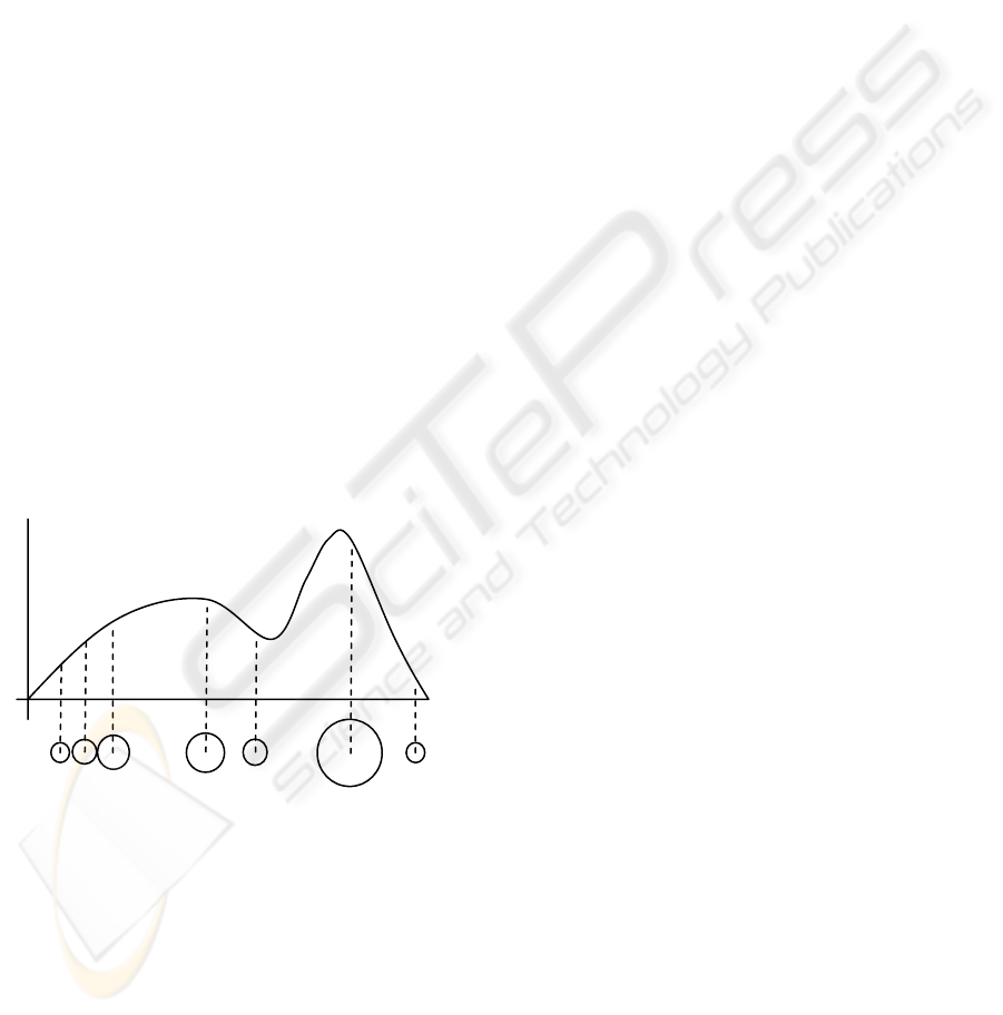
Figure 1: Representing a continuous PDF using a particle

set of 7 particles. The particles are randomly distributed,

and the weight of a particle (represented by the size of the

circle) corresponds to the value of the function at that

point.

As shown in Figure 1, a continuous function can be

approximated by a finite number of particles and

their weights. The more particles that are used, the

more accurate the representation. Normally, when

tracking a moving object, the PDF is a measure of

the probability of the target actually being at a

position, and is measured using an observation

model which reports high probabilities when it is

over an area of image that matches the target

appearance model. So, in Figure 1 above, the first,

lower peak might represent the location of some

background clutter, and the second, higher peak the

actual target.

When tracking a target over time, the predicted

position of the object depends on both where the

object was at the last timestep, and on a motion

element determined by a dynamic model of the

target. Propagating the continuous PDF estimate of

position forward in time with this motion model

tends to shift the curve in the direction of the

prediction. Adding an additional random diffusion

term, simulating noise in the tracking, has the effect

of smoothing the PDF, and after the motion phase,

the PDF is reinforced with measurements using the

observation model.

In the discrete case, where a finite set of particles

represents the distribution, a set of particles are

selected and have the motion model applied to their

state. These particles are selected with a probability

in proportion to their weight, and are replaced after

selection, ready for re-selection. This has the effect

of generating a new particle set in which the

particles tend to cluster mainly around the higher

probability peaks, with fewer particles representing

the lower probability valleys. As the peaks are what

we are interested in (they suggest where our target

actually is), this importance sampling improves

tracking performance.

This process is known as factored sampling.

Every time we select a particle we process its state

parameters forward in time using the motion model,

and then weight this particle based on the

observation model at this new position. This gives us

our new set of weighted particles, ready for another

iteration of the algorithm. One of the attractions of

particle filtering methods is that the sample set size

remains constant, so the algorithm runs in a

predictable time, and the quality of the

representation of the PDF can be increased by

increasing N, the number of particles in the set. A

classic example of a computer vision tracking

algorithm which uses an algorithm like this is the

Condensation algorithm (Blake & Isard, 1998).

We have adapted this tracking model so that

instead of being used over time, it is used over

space, to trace along a root in a digital image. It is

assumed that the root lies approximately parallel to

one of the major image axes, so we know

approximately which way to trace the image. We

shall assume here that the root lies approximately

parallel to the y-axis.

The algorithm proceeds as follows:

(

)

A PROBABILISTIC TRACKING APPROACH TO ROOT MEASUREMENT IN IMAGES - Particle Filter Tracking is

used to Measure Roots, via a Probabilistic Graph

109

1. The user selects, in the image plane, the starting

point of the root to be traced. Around this an

initial distribution of N particles is built. This

distribution is normally a Gaussian distribution

along the x-axis, centred on the user’s click

point. The y-locations are fixed to the user’s set

y-coordinate for reasons which will become

clear. Initially all these particles are given equal

probability weights.

2. Particles are selected with replacement in

proportion to their probability weighting. As

each particle is selected, its y-coordinate is

incremented by exactly 1 pixel, and the x-

coordinate is processed forward using its

predictive ‘motion’ model plus a small level of

random Gaussian noise.

3. The new particles are weighted by comparing

the image at their current location with the

observation model of a root cross section.

4. The probabilities associated with each particle,

and the locations of the particles are stored as

nodes in a graph – this will be used later on. All

the nodes at time t are connected to all the nodes

at time t-1, therefore each iteration N new nodes

and N*N new edges are added to the graph.

5. The algorithm repeats to step 2, until the root is

fully traced and the user stops the process at

iteration I.

Fixing the y-coordinate to proceed at an increment

of 1 pixel per iteration provides an external force to

the tracing algorithm to move the trace down the

root by exactly one pixel at a time. This is analogous

to tracing a line by hand using a pencil, starting at

one end and moving smoothly to the other. This

external force along the y axis, combined with the

motion model to cope with curvature along the root

in the x axis, replaces the motion model used when

tracking moving objects, and allows an

uninterrupted and unrepeated line to trace along the

root.

At the completion of the algorithm, there exists a

graph G with N*I nodes and N*N*I edges. Each

node represents a weighted sample from the particle

filter, and has a corresponding weight (probability),

and coordinate within the image plane. An example

visualization of how the graph relates to the particles

and image is presented in Figure 2.

It should be noted that currently the tracing is

ended manually by the user when the trace is seen to

reach the end of the root. Detecting when tracking

should cease is a hard problem as tracking

algorithms assume the target to exist at the next

timestep. The authors are working on a robust

method to detect the end of the root automatically,

which is mentioned further in Section 4.1.

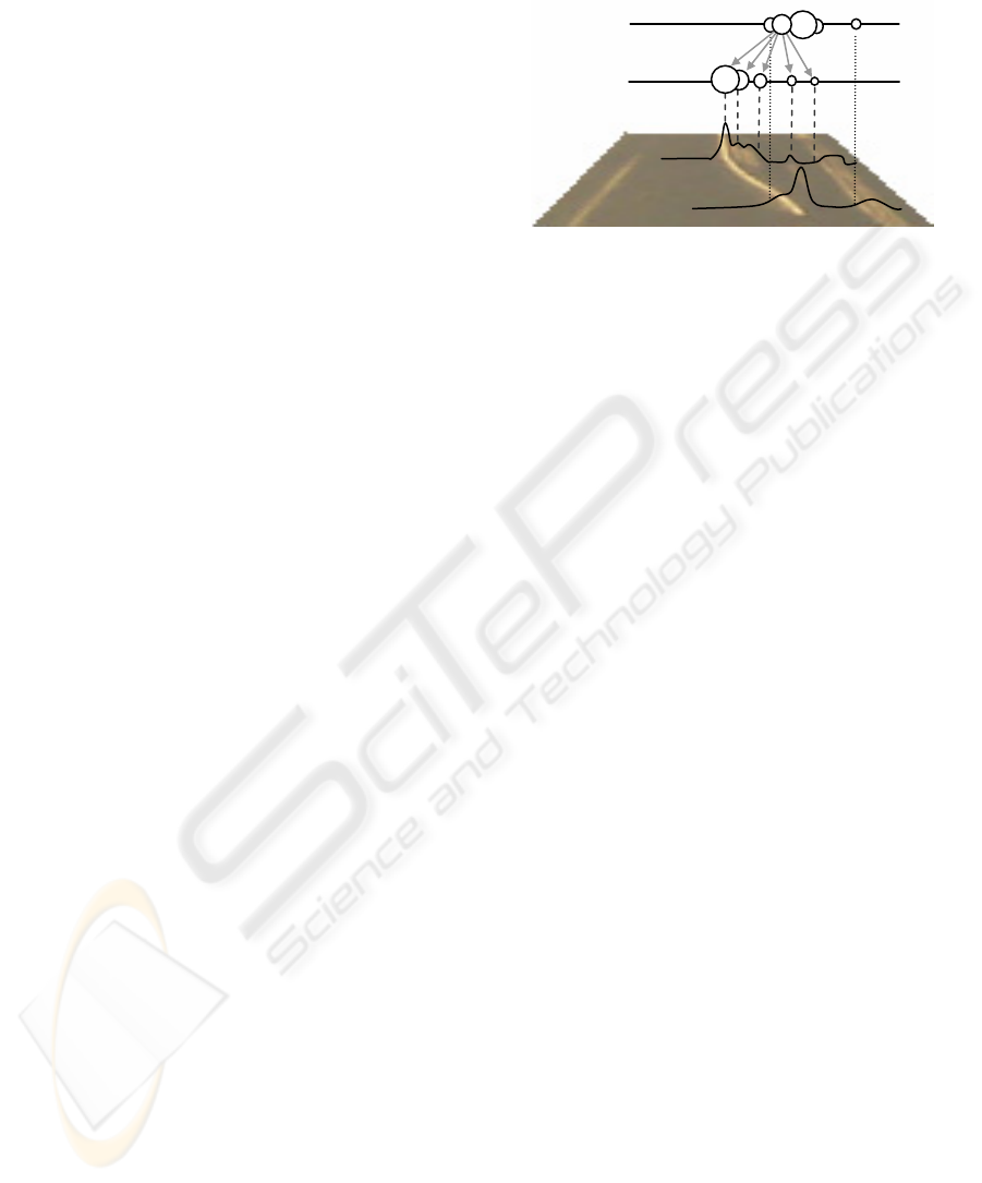
Figure 2: Illustration of the relationship between the

images, observation model output (curves), particle

weights (circles), and graph connections between two

steps in the algorithm, t and t-1. Note some of the lines

connecting the curves to particle weights at t-1 have been

omitted for clarity. Grey arrows indicate the edges from

one particle when it is mapped to a node in the graph– in

fact every node at each layer has edges connecting to all

nodes generated at the next step of the algorithm.

2.2 Probabilistic Graph

Graph G can be thought of as a 3D surface map

which represents probabilities associated with each

possible root location. Using this we aim to produce

an accurate measure of root length. This is done by

removing low probability nodes from the graph and

then finding the minimum distance route through the

remaining graph, from the start position to an end

node.

Low probability nodes are removed as they

represent areas of the image space explored by the

particles which are not centred over the root. During

the root tracking procedure, at each iteration

particles are spread around the root width, to

increase the chances of finding the root at each step.

The aim of our graph pruning procedure is to

remove those nodes from the graph that represent

locations in the image which are so far from the

ideal observation model result that they cannot

represent a root location. This information is useful

during the online tracking, but is not needed for the

offline graph traversal.

To do this pruning, we simply remove

probabilities whose measurements fall below a

certain number of standard deviations from the mean

measurement across the set, although any heuristic-

based method could be employed here to remove

low quality nodes from the graph. This has the effect

of producing a leaner graph which only covers the

space occupied by the root.

To actually find the shortest path through the

graph, Dijkstra’s method for determining shortest

-1

BIOSIGNALS 2008 - International Conference on Bio-inspired Systems and Signal Processing

110

paths was implemented. This method involves a

greedy algorithm which determines the shortest

distance to each node as it traverses the graph, in our

case along the length of the root, therefore giving the

shortest path along the length of the root, through

the remaining high-quality nodes.

3 RESULTS

The proposed method was tested by comparing

measurements of roots obtained using standard

manual techniques and using the new software. The

particle filter used 25 particles in all the tests.

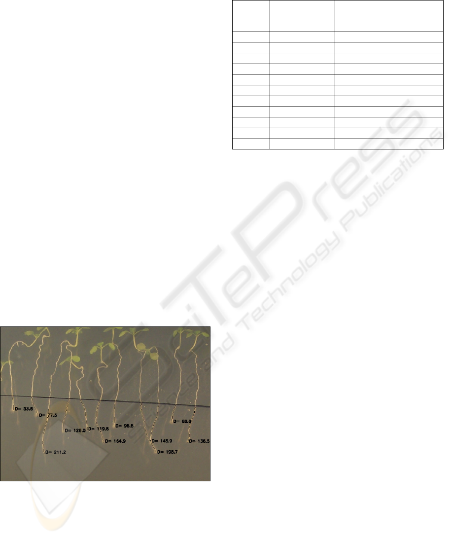
3.1 Software versus Non-expert User

The software was tested with an image of plated

roots (Figure 3). The aim was to measure the length

of the roots from the black line to the root tip. The

image had been taken with an off the shelf digital

camera, and was stored in a compressed JPEG

format, at a resolution of 783x576 for the close-up in

Figure 3. The roots were measured manually, by an

inexperienced user, using the measure tool in ImageJ

(Abramoff et al., 2004). This measurement was

repeated 5 times. The particle-filter software was

also run five times. An example output is presented

in Figure 3, while numerical results are given in

Table 1.

Figure 3: Image of growing roots with the software output

overlaid. The root numbers refer to the results in Table 1.

Table 1: Results of a comparison between the new

software and manual measurements made by a non-expert.

Root Error between

means, pixels

Relative error

(Mean-mean error as % of

manual measure)

1 -0.1 0.18

2 1.26 1.65

3 3.16 1.52

4 1.3 1.02

5 2.14 1.84

6 2.12 1.29

7 3.86 4.1

8 4.36 2.23

9 1.58 1.05

10 1.98 2.96

11 1.84 1.35

The mean length for these roots is 126.4 pixels, from

the ground truth. The average standard deviation for

the manual measures was 1.97 pixels, and 1.71

pixels for the proposed software.

The average time taken to measure manually the

roots on the plate in Figure 3 once each was 112

seconds. The new software, including the time for

user interactions clicking on the image and stopping

the tracing, took 70 seconds.

The average relative error from Table 1 is 1.7%.

Root 7 produces the most ambiguous measures from

the new software, but on inspection its root tip is

blurry and ambiguous in the image itself, which may

explain the error. This situation might produce

measurements with high variability when different

subjects are asked to perform the measurement

manually.

3.2 Software versus Expert User

The software was also tested against manual

measurements made by an expert user. The root

images used in this section are more complex, with

the roots showing many lateral roots. There are also

significant reflections from the rear of the plate, and

the images are of low resolution (640x480), all of

which makes this scenario a challenge for the

software.

For this experiment, five roots in Figure 4 were

manually measured in ImageJ by a trained biologist

familiar with making such measurements. This

measurement was compared with the average results

of five runs of the new software approach. The data

is presented in millimetres; using the ruler in Figure

3 a conversion was calculated between pixels and

millimetres. The results are presented in Table 2.

The test image is presented in Figure 4.

1 2 3 4 5 6 7 8 9 10 11

A PROBABILISTIC TRACKING APPROACH TO ROOT MEASUREMENT IN IMAGES - Particle Filter Tracking is

used to Measure Roots, via a Probabilistic Graph

111

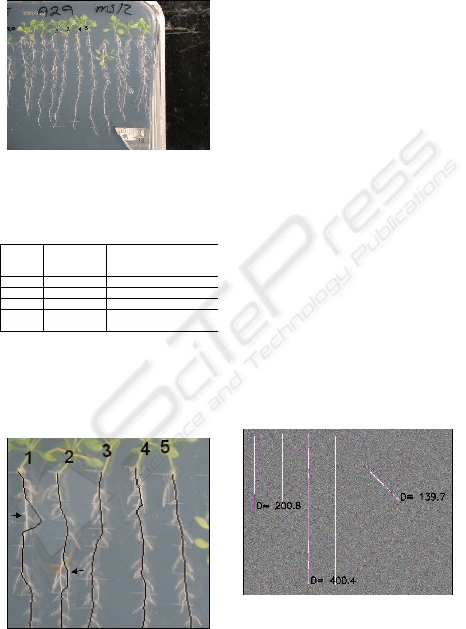
Figure 4: Image of growing roots. Note the large numbers

of lateral roots and reflections which clutter the image.

The root numbers refer to the results in Table 2.

Table 2: Results of a comparison between the new

software and manual measurements made by an expert

user.

Root Error

between

means, mm

Relative error

(Mean-mean error as % of

manual measure)

1 0.78 1.67

2 -1.95 4.54

3 1.32 2.89

4 0.86 1.81

5 0.02 0.05

The average root length from the manual measures

was 46.8mm. The proposed software measures had

an average standard deviation of 0.23mm. The

average relative error from Table 2 is 2.2%.

The automatic tracing of roots 1 and 2 suffered

the most due to interference from the lateral roots.

Examples of such error cases are presented in Figure

Figure 5: Example output, with error cases marked.

Figure 5 illustrates two of the most common error

cases. For case (a), the lateral root is followed rather

than the main root about 50% of the time. This is

because when tracing the line, the tracking algorithm

reaches a junction, and as the motion model predicts

the line to continue roughly half way between the

two actual lines, and both lines produce very similar

measurement models, half the time the algorithm

will take one route, and the other half of the time the

other route will be followed.

The particle filtering trackers can cope with this

kind of ambiguity over short distances, but over

longer distances the samples tend to all migrate to

the hypothesis which is producing the slightly better

observation measures at the time. This fading of a

hypothesis is a common practical problem with

particle filter tracking (King & Forsyth, 2000).

In error case (b) in Figure 5, the error is caused

by the lateral root consistently having a better

measurement model. This error will therefore be

present on every run of the algorithm. On inspection,

the better measurement appears to be caused by a

misrepresentation of the main root in the image. The

root here appears very thin. This may be an artefact

introduced by the low resolution of the image.

However it is caused, the result is that the lateral

root provides a higher response to the measurement

model and hence the root is traced along this

erroneous path.

3.3 Artificial Scenarios

The software was also tested against artificial

images. These images were produced using straight

lines of a similar colour to the roots. Gaussian noise

was applied to the image.

Figure 6: An artificial image with lines of length 200, 400

and 141.4 pixels respectively. Overlaid are example

measurements produced by the new software.

BIOSIGNALS 2008 - International Conference on Bio-inspired Systems and Signal Processing

112

The purpose of this experiment was to test the

software against a known ground truth measurement.

Figure 6 shows one result out of 5 repeats which

aimed to test the measuring software against a

simple artificial ground truth. The results for the 3

lines measured are presented in Table 3.

Table 3: Results of running the algorithm on artificial data.

Line True

length

(pixels)

Average measured

by new algorithm

(pixels)

Average

error

(pixels)

1 200 199.9 -0.1

2 400 400.2 0.2

3 141.4 140.3 -1.1

4 SYSTEM EXTENSIONS

The basic system described and tested above has

been extended in two ways. First, a method is being

developed to automatically detect when the end of

the root has been reached. Second, a mixed state

particle filter (Isard & Blake 1998) has been

incorporated into the framework to allow the

labelling of different possible growth modes for the

root, such as a gravitropic response. These will be

described below.

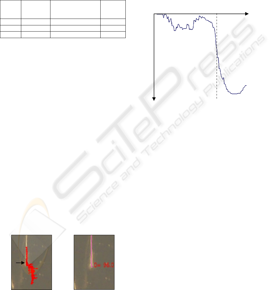
4.1 Automatic Root Tip Detection

One of the major time consuming and error prone

aspects of the root measurement system detailed

above is the manual intervention required to stop the

line tracing when the end of the root is reached.

This was necessary because the premise of the line

tracker is that at each iteration the next point on the

line definitely does exist somewhere in the image –

this assumption is broken when the end of the root is

reached. In the absence of a tip detection capability

or manual input the tracker will trace whatever

produces the best measurement from the image, e.g.

see Figure 7 (left).

The developed method proceeds as follows. During

the line tracing phase of the software, the user

allows the system to track beyond the end of the

root. The graph traversal then proceeds as before,

and a final path representing the trace of the root is

produced. Now the new step: the measurement

probabilities along this path are examined. Figure 8

below shows the trace of log probabilities along a

root:

Figure 8: Graph depicting how log of measurement

observation probabilities varies along the root. The dashed

line marks the approximate end of the root.

Summary statistics of the log probabilities are

calculated along the chosen path, and the end of the

root is marked as where the current measurement

falls below a set number of standard deviations from

the mean. This was seen to work well on 7 of the 11

roots in Figure 3 – see figure 7 (right) for an

example output.

4.2 Labelling of Growth Modes

It is possible to build into the existing particle

filtering framework more than one predictive model

to process the particles forward along the root

image. This is achieved using a form of mixed state

particle filter (Isard & Blake, 1998). Essentially, it

is possible to define multiple models for the driving

force behind the tracing of the root, and the most

appropriate of these will generate higher quality

particles at each step. For example, to model

gravitropic growth, one model might aim to trace the

root left to right across the image, and the second

model would aim to trace the root top to bottom.

Whichever model prospered the most is naturally

selected to label the image – see Figure 9.

Distance along roo

0 Log (p) -8

Figure 7: Left: A particle filter tracker will always try and hunt

target even if one does not exist, as the spread of particles past the

root tip (indicated by arrow) shows. Right: An example result o

the same root image with the new root termination criteria

A PROBABILISTIC TRACKING APPROACH TO ROOT MEASUREMENT IN IMAGES - Particle Filter Tracking is

used to Measure Roots, via a Probabilistic Graph

113

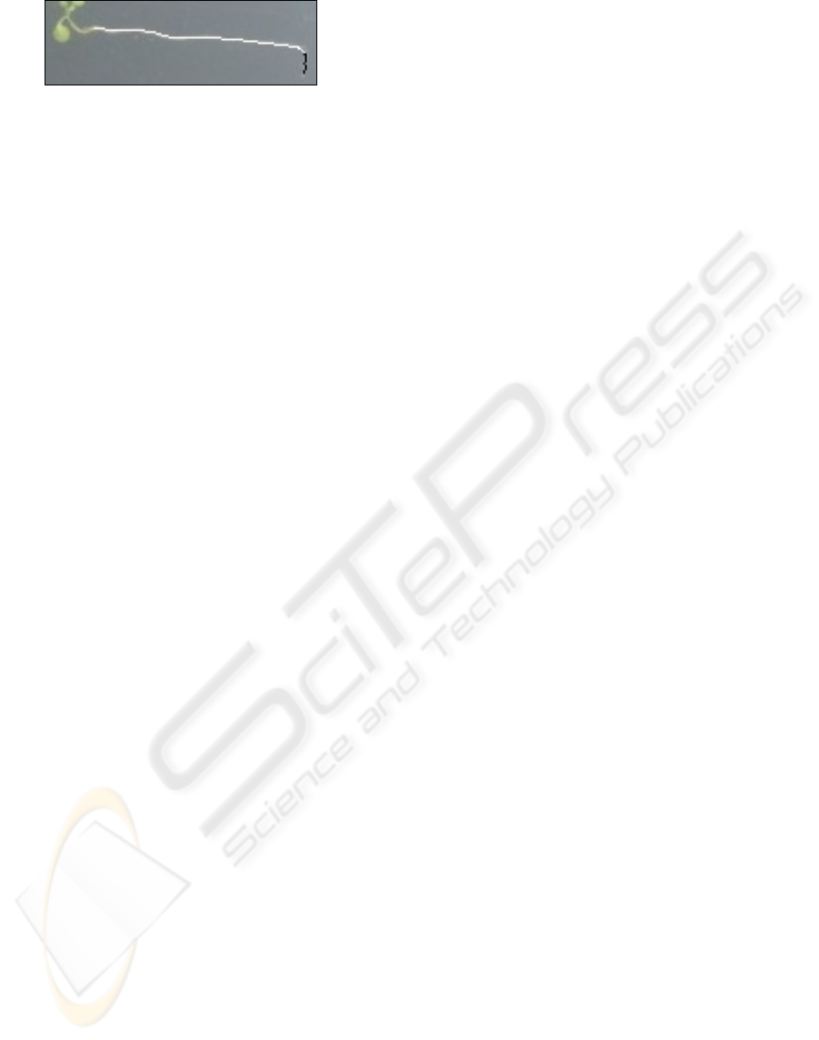
Figure 9: Example root trace using a mixed state model

consisting of two states, normal growth (white) and

gravitropic (black).

5 CONCLUSIONS

5.1 Discussion of Results

The results comparing the software root length

measures to the manual measurements show the new

technique to produce results to about 2% of the

actual measures most of the time. There was a

larger error when comparing the new software with

the expert user (2.2%) compared to the non-expert

(1.7%), however the images in Section 3.2 are more

challenging than those in Section 3.1, which may

account for some of the increased error also.

Something to be wary of with these kinds of

comparisons is using manually marked-up ground

truths to compare with the automated measurements.

There is an inherent subjectivity in determining the

length of the roots, dependant on, for example, the

accuracy with which the curves in the roots are

traced. The more finely the shape of the root is

followed, the longer the measurement. There is

similarity here with the coastline measuring

problem. Some structures can be thought of as

fractal in composition, such as a coastline

(Mandelbrot, 1967) or complete root systems (Eshel,

1998). When trying to measure such systems, the

scale (or accuracy) with which the waves and

perturbations are traced has a bearing on the overall

length calculated. This software can be thought of as

producing the finest scale estimate of length

available at the image resolution, and so is likely to

overestimate length compared to a manual

measurement. This may be reflected in the results

reported in Section 3, with most errors indicating an

overestimate of line length.

Even if a user and the new software were to use

the same scales of measurement, there is still human

error present in the measuring process, which can be

quantified by the standard deviation of the manually

measured data. The manual measurements in section

3.1 give an average standard deviation of ~2 pixels.

Therefore most (99%) of the manually measured

lengths can be expected to fall within about 6 pixels

(three standard deviations) of the true value for roots

of around the length seen in section 3.1. The new

software used on these roots has an average relative

error of 1.7% which translates to a error of 2.1 pixels

on average for these roots, and therefore this

software error falls within the expected error bounds

of manually entered data.

The time to use the new software was less than

the time to take the measurements manually. This

should be improved upon still when implementation

of the root tip finding algorithm is completed. The

system should be less fatiguing to the user as less

high-accuracy input is required. This will help to

lower the number of mistakes made over the course

of measuring many roots.

Labelling of the different growth modes of the

root as illustrated in Section 4.2 is also ongoing

work, but early results indicate the system can be

used for identifying different ways in which a root

trace line is produced, as long as trace motion

models exist to sufficiently differentiate the modes

of production of the line.

5.2 Improving the Reliability

As it stands, the software is still in trial stages and

reliability is still being improved. There are a

number of possible ways to decrease the number of

errors that can occur. One problem is as the particle

filter tracks the root towards the tip, it is liable to

trace lateral roots if they are long enough and

provide a high enough quality measurement, as

shown in Figure 5. A simple way to remove this

problem is to simply trace the root from the end tip

upwards. Due to the geometry of the lateral roots the

tracing algorithm is then not presented with viable

alternative routes until the lateral roots join and

terminate. Therefore, the only way they can be

followed is if they lie parallel to the main root for

long enough, and are close enough for the particles

on the tracing algorithm to ‘jump’ across to the other

track. The difficulty with this approach, however, is

that the tracker would have to be started on the

thinnest, least visible section of the root, which may

be hard to detect, and automatic termination of the

tracking becomes harder as the delineation at the top

of the root is less clear.

Other general improvements include increasing

the resolution of the images, as during testing at

least some of the mis-tracing of the roots was due to

poor representation of the roots in the image.

Improving the measurement model may lead to less

problems with the system tracking lateral roots.

Finally, increasing the number of samples may be

beneficial, especially in combination with greater

image resolution. However, in such a case speed of

BIOSIGNALS 2008 - International Conference on Bio-inspired Systems and Signal Processing

114

traversal of the graph, which currently is near

instantaneous, might become a limiting factor.

5.3 Future Potential of the System

The particle filter approach, with or without mixed

state extensions, provides a general framework for

matching models of elongated structures to images

of those structures. By changing the models used it

may be possible to extract descriptions of and

measure a wide variety of roots and other plant

components. In particular, given higher resolution

(e.g. confocal) images showing the cellular structure

of the plant, it may be possible to predict (using the

motion model) and detect (using the appearance

model) higher level structures such as files of cells

of similar type.

The ability to recognise state changes by using a

mixed state, rather than pure particle filter, also

raises the possibility of recognising a wide variety of

events during plant growth, of which the onset of

gravitropic response may be just the first.

REFERENCES

Abramoff, M. D., Magelhaes, P. J., & Ram, S. J. (2004).

Image processing with ImageJ. Biophotonics

International, 11, 36-42.

Bauhus, J. & Messier, C. (1999). Evaluation of fine root

length and diameter measurements obtained using

RHIZO image analysis. Agronomy Journal, 91, 142-

147.

Blake, A. & Isard, M. (1998). Active Contours. (Second

ed.) Springer-Verlag.

Eshel, A. (1998). On the fractal dimensions of a root

system. Plant, Cell and Environment, 21, 247-251.

Isard, M. & Blake, A. (1998). A mixed-state

CONDENSATION tracker with automatic model-

switching. Proc 6th Int.Conf.Computer Vision, 107-

112.

King, O. & Forsyth, D. A. (2000). How does

CONDENSATION behave with a finite number of

samples? Proc.ECCV 2000, 695-709.

Mandelbrot, B. B. (1967). How long is the coast of

Britain? Science, 156, 636-638.

Pateña, G. F. & Ingram, K. T. (2000). Digital image

acquisition and measurement of peanut root

minirhizotron images. Agronomy Journal, 92, 544.

Qi, X., Qi, J., & Wu, Y. (2007). RootLM: a simple color

image analysis program for length measurement of

primary roots in Arabidopsis. Plant Root, 1, 10-16.

Smucker, A. (2007). WR-RIPL 2.0.

http://rootimage.css.msu.edu/WR-RIPL/index.html

Accessed 20-6-2007.

A PROBABILISTIC TRACKING APPROACH TO ROOT MEASUREMENT IN IMAGES - Particle Filter Tracking is

used to Measure Roots, via a Probabilistic Graph

115