A FEATURE GUIDED PARTICLE FILTER FOR ROBUST HAND
TRACKING
Matti-Antero Okkonen
VTT Technical Research Centre of Finland, P.O. Box 1100, FI-90571 Oulu, Finland
Janne Heikkil¨a, Matti Pietik¨ainen
Department of Electrical and Information Engineering, P.O. Box 4500, FI-90014, University of Oulu, Finland
Keywords:
Particle filtering, hand tracking, importance sampling, adaptive color model.
Abstract:
Particle filtering offers an interesting framework for visual tracking. Unlike the Kalman filter, particle fil-
ters can deal with non-linear and non-Gaussian problems, which makes them suitable for visual tracking in
presence of real-life disturbance factors, such as background clutter and movement, fast and unpredictable
object movement and unideal illumination conditions. This paper presents a robust hand tracking particle
filter algorithm which exploits the principle of importance sampling with a novel proposal distribution. The
proposal distribution is based on effectively calculated color blob features, propagating the particles robustly
through time even in unideal conditions. In addition, a novel method for conditional color model adaptation
is proposed. The experiments show that using these methods in the particle filtering framework enables hand
tracking with fast movements under real world conditions.
1 INTRODUCTION
Visual hand tracking is an important part of the grow-
ing field of automatic human activity recognition.
Hand gestures are a natural part of human commu-
nication and automatic interpretation of them would
have numerous applications, for example in natural
user interfaces, in automatic sign language recogni-
tion, in virtual reality and even in emotion recog-
nition. In addition, visual tracking of hands offers
a non-contact modality, where no special hardware
is needed. However, in order to work in real en-
vironments, tracking algorithms must tackle convo-
luting factors such as fast and complex hand move-
ments, changing object appearance, unideal illumina-
tion conditions and background movement and clut-
ter.
Previous work on hand tracking can be divided by
how the hand is modeled: Some approaches treat the
hand as a deformable object and try to solve the pa-
rameters that define the hand’s articulation, whereas
other methods aim for bare trajectory information by
estimating the spatial location of the hand through
time. The earliest attempts for hand tracking used
data gloves or visual markers for the task, but grad-
ually the focus moved to purely visual based systems,
such as the DigitEyes (Rehg and Kanade, 1993). An-
other important milestone in this field was the intro-
duction of particle filtering for visual tracking, which
was done by Isard and Blake with the Condensa-
tion algorithm (Isard and Blake, 1996). Particle fil-
ters are sophisticated statistical estimation techniques
that can deal with non-linear and non-Gaussian prob-
lems, which makes them well suited for visual track-
ing. Many variations of the basic particle filtering
algorithms have been proposed for both spatial and
articulated hand tracking since the Condensation al-
gorithm. More information about the earlier work on
hand tracking can be found in (Pavlovic et al., 1997;
Mahmoudi and Parviz, 2006).
In spatial hand tracking, a group of methods have
augmented the basic particle filtering algorithms with
an enhancement step, where the spatial locations of
the particles are improved using some optimization
technique. Pantrigo et al. have used the local search
and the scatter search algorithms (Pantrigo et al.,
2005b; Pantrigo et al., 2005a), whereas Shan et al.
have utilized the Mean Shift algorithm (Shan et al.,
2004). The last-mentioned method exploits mean
shift with color and motion cues for all particles in
368
Okkonen M., Heikkilä J. and Pietikäinen M. (2008).
A FEATURE GUIDED PARTICLE FILTER FOR ROBUST HAND TRACKING.
In Proceedings of the Third International Conference on Computer Vision Theory and Applications, pages 368-374
DOI: 10.5220/0001078503680374
Copyright
c
 SciTePress

each time step. An optimization approach have also
been proposed to articulated hand tracking by Lin et
al. using the Nelder Mead algorithm (Lin et al., 2004).
These optimization techniques aim for more efficient
use of the particles by relocating them to spaces where
they get bigger weights, thus reducing the variance of
the state estimate and enabling tracking with fewer
particles.
In this paper, a particle filtering algorithm for spa-
tial hand tracking is proposed. The algorithm em-
ploys a feature based proposal distribution for optimal
grouping of the particles through time. This way the
particles can be propagated based on current obser-
vations rather than a predefined dynamic model and
therefore there is no need for an additional indeter-
ministic optimization scheme as in (Pantrigo et al.,
2005b; Pantrigo et al., 2005a; Shan et al., 2004; Lin
et al., 2004). Furthermore, the impoverishment of
the particles can be avoided by adjusting the vari-
ance of the proposal distribution, which is not pos-
sible with the methods relying on the optimization
schemes. The proposal distribution is built on color
cue, since it is more perennial compared to motion
and edge information that may not always be observ-
able due to e.g. motion blur or lack of motion. In ad-
dition, a novel technique for color model adaptation is
presented, which restrains the model to falsely adapt
to background when tracking temporally fails, which
is largely ignored by previous methods. The proposed
method is referred as the Feature Guided Particle Fil-
ter (FGPF) troughout the paper.
The rest of the paper is organized as follows. Sec-
tion 2 gives an overview about the theoretical basis of
particle filtering and Section 3 explains the proposed
method in detail. Section 4 reports the experimen-
tal results, and finally, discussion and conclusions are
given in Section 5.
2 PARTICLE FILTERING
Particle filtering arises as an approximate solution to
the sequential Bayesian estimation framework. The
underlying problem is to estimate the pdf of hidden
parameters x
t
at discrete time steps, given a set of ob-
servations z
1:t
= {z
1
,...,z
t
}.
2.1 Recursive Bayesian Filter
In the Bayesian approach the posteriori pdf p(x
t
|z
1:t
)
is obtained recursively in two steps. In the prediction
step, the prior pdf is created by predicting the distri-
bution from the previous step
p(x
t
|z
1:t−1
) =
Z
p(x
t
|x
t−1
)p(x
t−1
|x
t−1
)dx
t−1
, (1)
which is updated in the update step when the current
observation is available
p(x
t
|z
1:t
) =
R
p(z
t
|x
t
)p(x
t
|x
t−1
)
p(z
t
|z
t−1
)
. (2)
Closed form solution exist to the problem in re-
stricted cases. The Kalman filter, for example, re-
stricts the model dynamics p(x
t
|x
t−1
) and the mea-
surement density p(z
t
|x
t
) to be linear and Gaussian.
Particle filter algorithms solve the above problem via
Monte Carlo simulations and rather than operating
with analytic expressions the distributions are repre-
sented with a set of discrete samples of the parame-
ter space (i.e. particles) {x
i
,w
i
}
N
S
i=1
, with associated
weights. Although particle filters only approximate
the solution, they can deal with non-linear and non-
Gaussian system and measurement models. Espe-
cially the ability to deal with arbitrary distributions is
an advantage when applying them to visual tracking
in cluttered environments. A more detailed introduc-
tion to particle filtering can be found in (Arulampalam
et al., 2002).
3 FEATURE GUIDED PARTICLE
FILTER (FGPF)
This section gives a detailed description of the pro-
posed method.
3.1 Object Model
The human hand is a complex object and modeling
its deformations leads inevitably to high-dimensional
models that require learning the model parameters
(Rehg and Kanade, 1993; Isard and Blake, 1996).
Since the goal here is to estimate only the location
of the hand, it is modeled with rectangles for their
generality and simplicity. The model consists of two
concentric rectangles, R
c
and R
m
, for evaluating both
the color and the motion cue, respectively. The di-
mensions of the model remain fixed throughout pro-
cessing, which leaves the state of the model to be de-
termined by the central coordinates
x = (x
c
,y
c
)
T
. (3)
3.2 Measurement Model
The measurement model is based on a fusion of color
and motion cues. Edge density is omitted here since
A FEATURE GUIDED PARTICLE FILTER FOR ROBUST HAND TRACKING
369

it requires detailed information about the object’s ge-
ometry and is easily degraded by motion blur.
Skin color forms a compact cluster in chromatic-
ity space, which makes it a popular feature for hand
tracking. In our approach, skin color is modeled
with a two dimensional histogram in (r,g) space of
Normalized Color Coordinates (NCC). This way the
model can present arbitrary distributions based purely
on chromatic values. Similar to (P´erez et al., 2004),
the color likelihood of a particle is defined as
p(z
c
|x) ∝ exp(−D
2
c
/2σ
2
c
), (4)
where
D
c
= 1 −
N
b
∑
r=1
N
b
∑
g=1
p
P(r,g)C(r,g) (5)
is built on the Bhattacharyya distance between the
object histogram P(r,g) and the color reference his-
togram C(r, g) in (r,g) color space.
The motion cue is computed by following the ap-
proach in (Shan et al., 2004) by evaluating the ab-
solute difference of luminosity between successive
frames ∆I
t
= |I
t
− I
t−1
|. Using this, a binary image
I
m
is computed, where each pixel I
m
(x,y) is assigned
with 1 if the average difference in the 3 × 3 neigh-
borhood of ∆I
t
(x,y) exceeds a predetermined thresh-
old T
m
and 0 otherwise. The motion likelihood of a
particle is defined as the color likelihood, where the
motion distance is defined as
D
m
=
1
A(R
m
)
∑
x,y∈R
m
I
m
(x,y). (6)
A(R
m
) denotes the area of R
m
in above equation.
Using the assumption that the color and motion
cues are statistically independent, the measurement
model can be seen as their product
p(z|x) ∝ exp(−D
2
c
/2σ
2
c
− D
2
m
/2σ
2
m
). (7)
3.3 The Proposal Distribution
The performance of a particle filtering algorithm is
dependent on how the particles are distributed in the
state space. Importance sampling is a technique used
in Monte Carlo methods that aims for assigning the
particles to spaces where the measurement density
is high (Arulampalam et al., 2002). This improves
efficiency and reduces the variance of the parame-
ter estimate since particles with small weights would
have negligible impact on the estimate. The idea
is to draw the particles from a proposal distribution
q(x
t
|x
t−1
,z
t
) that can exploit currentmeasurements z
t
rather than using the predetermined prior p(x
t
|x
t−1
).
Here, a color based proposal function for efficient
distribution of the particles is presented. Color is cho-
sen because it is more permanent than motion and
gradient cues, that can be easily lost due lack of mo-
tion or motion blur. Furthermore, the use of gradient
information would require object shape information,
which would complicate the system beyond the ob-
jectives of the spatial tracking. To make the color cue
as discriminative as possible, the color model is cre-
ated from a small portion of the object and is updated
along the image sequence. Color based blob features
havebeen earlier used in articulated hand tracking, for
example, for evaluating the object likelihood (Bret-
zner et al., 2002). Color segmentation has also been
used as a coarse level proposal distribution in (Isard
and Blake, 1996).
To create the proposal function, first a color like-
lihood image I
c
is created from the color model
C(r,g) by histogram backprojection (Swain and Bal-
lard, 1991). The blobs are detected from the likeli-
hood image following the method of (Bretzner and
Lindeberg, 1998) by evaluating the squared Laplacian
∇
2
L(x,y) =
∂
2
∂x
2
L(x,y) +
∂
2
∂y
2
L(x,y). (8)
where L(x,y) = g(·) ∗ I
c
(x,y) and g(·) is a Gaussian
kernel. The partial derivatives
∂
2
∂x
2
L(x,y) can be ex-
pressed as a convolution of
∂
2
∂x
2
g(·) with the likeli-
hood image I
c
(x,y). Straightforward application of
the convolution would be computationally demand-
ing, which is avoided here by approximating the sec-
ond order derivative Gaussian
∂
2
∂x
2
g(·) with box filters,
as in the SURF descriptor (Leonardis et al., 2006).
This way the convolution can be computed very fast
using integral images. For detailed descriptions about
the box filters and the integral images, we refer to
(Leonardis et al., 2006) and (Viola and Jones, 2001),
respectively.
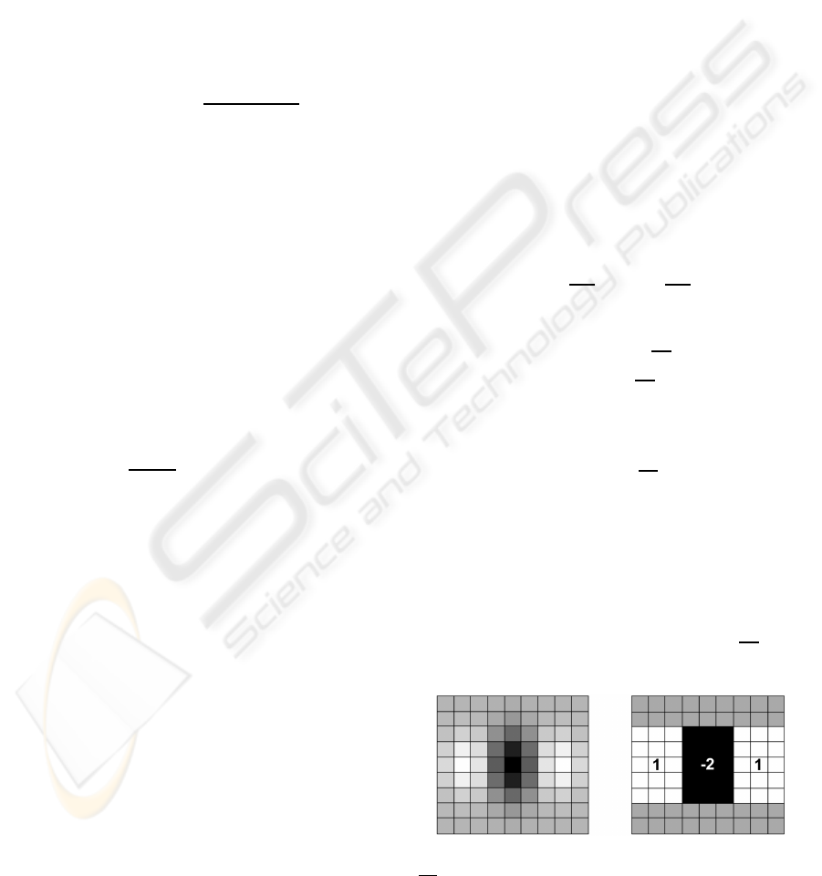
As an illustration, a 9 × 9 box filter approxima-
tion of the second order Gaussian derivative
∂
2
∂x
2
g(·) is
shown in Fig. 1.
Figure 1: A cropped second order gaussian derivative
∂
2
∂x
2
g(·) and its box filter approximation.
However, in practice the filter size must be consid-
VISAPP 2008 - International Conference on Computer Vision Theory and Applications
370

erably larger for detecting hand sized blobs. Note that
the computational burden of convolution is invariant
to the size of the box filter.
The blobs are detected as local maxima in
−∇
2
L(x,y), yielding in a set of blob centers
B = {c
i
b
,ξ
i
}
N
b
i=1
(9)
corresponding to weights ξ
i
∝ −∇
2
L(c
i
b
). Points with
weights smaller than a given threshold T
b
are consid-
ered insignificant and are therefore excluded from the
set.
The dynamicsof the system is modeled with a sec-
ond order autoregressive model
x
t
= 2x
t−1
− x
t−2
+ υ, (10)
where υ equals to Gaussian noise component with
zero mean and variance σ
d
. The model is kept simple
to achieve a level of generality, since human hand mo-
tion can be diverse and learned models are inevitably
biased to their training data.
Finally, the proposal distribution is defined as
q(x
t
|x
j
t−1
,x
j
t−2
,B
t
) ∝
N
b
∑
i=1
ξ
i
p(c
i
b
|x
t−1
j
,x
j
t−2
)N (x
t
;c
i
b
,σ
2
p
I)
(11)
where N (·) and I denote isotropic Gaussian distribu-
tion and identity matrix, respectively, and p() stands
for the dynamic model. Using blob features, the parti-
cles are distributed around skin colored areas. In addi-
tion, the Gaussians in (11) are weighted not only with
the blob weights ξ
i
, but also with the dynamic model
to favor blobs that induce smoothness into the particle
trajectories. Note that both the proposal distribution
(11) and the measurement density (7) need to be de-
fined only up to proportionality (Arulampalam et al.,
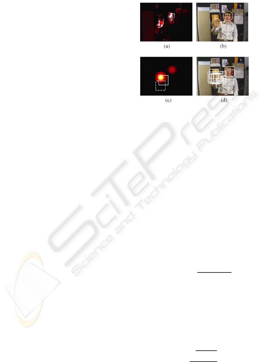
2002). An illustration of the proposal distribution is
given in Fig. 2.
3.4 Location Estimate and Color Model
Adaptation
As stated in Section 2, the posterior pdf is not nec-
essary unimodal. This situation arises often when
the background contains clutter and additional move-
ment. In such cases the location estimate calculated
as the weighted mean of the particles is biased by the
”outlier particles”. To avoid this, the location estimate
is calculated here as a weighted mean of a subset

{x
′
,w
′
} ∈ {x,w} : ||x
′
−
ˆ
x|| < R
e

, (12)
Figure 2: Illustration of the proposal distribution. (a) A
color likelihood image I
c
at time t and (b) the detected
blobs, marked with circles. (c) The proposal distribution for
an individual particle, where the continuous and the dashed
rectangles mark the state of the particle at t − 1 and t − 2
respectively. (d) The resulting particle set.
where
ˆ
x equals to the particle in the full set {x,w}
with the biggest weight and R
e
defines the radius of
the area from which the subset is collected.
In each time step, a color histogram H
t
(r,g) is
computed in the Normalized Color Coordinates from
the pixels inside the smaller object rectangle R
c
of
the location estimate. The histograms are stored in a
buffer of length N
buf f
, from which the reference color
model C
t
(r,g) is composed as their mean, following
smoothly the changes in the hand’s appearance. If the
location estimate should fail, the color model should
not be adapted. To recognize such events, two steps
are taken: In the first step, the candidate histogram
H
t
(r,g) and the current reference model C
t
(r,g) are
tested for similarity using the Bhattacharyya distance
D(H
t
,C
t
) =
N
b
∑
r=1
N
b
∑
g=1
p
H
t
(r,g)C
t
(r,g). (13)
The candidate is added to the buffer only if
D(H
t
,C
t
) > τ
c
. An abrupt change between the current
reference and the candidate is taken to be an indica-
tion of a false estimate. The second step is to evaluate
the amount of ambiguity which each new histogram
H
t
(r,g), that passes the first step, adds to the model.
For every frame, a scatter measure for the likelihood
image I
c
is computed as
S (I
c
) =
q
µ
′
2
20
+ µ
′
2
02
X ·Y
, (14)
A FEATURE GUIDED PARTICLE FILTER FOR ROBUST HAND TRACKING
371

where X and Y denote the dimension of the image.
The moments µ
′
20
= µ
20
/µ
00
and µ
′
02
= µ
02
/µ
00
are
constructed from central moments
µ
pq
=
∑
x
∑
y
(x− x)
p
(y− y)
q
I
c
(x,y), (15)
where (x,y) is the center of gravity of the image.
Since the size of the hand should not change too much
between consecutive frames, a sharp increase in the
scatter of the color likelihood image is considered to
be caused by a false estimate. Thus, if S
t
− S
t−1
> τ
s
,
the previouslyadded histogram H
t−1
(r,g) is discarded
from the buffer. This situation occurs, for example,
when the model falsely adapts to an background ob-
ject that meets the condition in the first step.
3.5 The Algorithm
According to the importance sampling theory, the par-
ticle weights must be augmented with a correction
factor when sampling from the proposal distribution.
As derived in (Arulampalam et al., 2002), the particle
weight update equation then becomes
w
i
t
∝ w
i
t−1
p(x
i
t
|x
i
t−1
,x
i
t−2
)
q(x
i
t
|x
i
t−1
,x
i
t−1
,z
t
)
p(z
t
|x
i
t
), (16)
where the factor p(x
i
t
|x
i
t−1
,x
i
t−2
)/q(x
i
t
|x
i
t−1
,x
i
t−1
,z
t
)
emphasizes particles toward the dynamic model. This
factor is omitted here since the proposal distribution
is considered to be a better representation of the true
state than the generic dynamic model, in which case
the factor would degrade the estimate calculated from
the particles. This has been shownin our experiments.
The hand tracking algorithm used in the experi-
ments is built on the Sampling Importance Resam-
pling (SIR) algorithm and is presented in Table 1.
Table 1: Feature Guided Particle Filter (FGPF) for hand
tracking.
To create the particle set {x
i
t
,w
i
t
}
N
p
i=1
, process each particle in the
previous set {x
i
t−1
,w
i
t−1
}
N
p
i=1
as follows:
1. Extract the feature set B = {c
i
b
,ξ
i
}
N
b
i=1
2. draw x
i
t
∼ q(x
t
|x
i
t−1
,x
i
t−2
,B )
3. update weight: w
i
t
∝ w
i
t−1
p(z
t
|x
i
t
)
4. Estimate the effective sample size
ˆ
N
ef f
=

∑
N
p
i=1
(w
i
t
)
2

−1
5. If
ˆ
N
ef f
< T
ef f
, draw x
∗i
t
∼ {x
i
t
,w
i
t
}
N
p
i=1
so that p(x
∗i
t
= x
j
t
) ∝
w
j
t
and replace {x
i
t
,w
i
t
} ← {x
∗i
t
,N
−1
p
}
6. Estimate the location of the object as the mean of the subset
defined in (12).
4 EXPERIMENTS
The experiments were made with a set of twelve test
sequences, where a user moved his hand randomly.
The sequences had 15 fps, a resolution of 320x240
and a mean length of 240 frames. Eight sequences
were made by varying three parameters: background
clutter (simple/cluttered), hand speed (slow/fast) and
the presence of the user (only the hand and arm in
the frames/user’s upper torso in the background). An-
other four sequences were made varying the first two
parameters, with the user and an additional person
moving in the background. Furthermore, to simulate
real-life incidents, the hand of the user occasionally
moved outside of the camera’s field of view for a few
frames. The center of the palm was manually labeled
as the reference point for each frame of the sequences.
For a comparison, the tests were performed
also with the Mean Shift Embedded Particle Filter
(MSEPF), implemented as presented in (Shan et al.,
2004). The parameters for the tests were found man-
ually for both methods, since global optimization over
the test sequences would have been infeasible. Each
parameteres was tested with few values and the op-
timal over all sequences was chosen. The selected
parameters are presented in Table 2. For the evalua-
tion, the average tracking rate was computed for both
methods, which is defined as the proportion of frames
where the estimate is within 20 pixels of the reference
point. Since both methods are stochastic in nature, the
tests were repeated 10 times for each sequence. Ta-
ble 3 shows the results for each sequence parameter
value, averaged over the others.
To verify the advantage of the presented proposal
distribution, the experiments were also performed by
replacing the proposal distribution with the dynamic
model. This produced an overall tracking rate of 0.65,
which is considerably lower than using the proposal
distribution. In addition, tests were also carried out
using the weighting equation (16), which yielded in
an overall tracking rate of 0.90.
As the results show, the presented method outper-
forms the MSEPF with the given parameters. The
tests showed that the Feature Guided Particle Filter
was able to deal with convoluting factors, such as
background movement and clutter with fast and di-
verse motion. Moreover, the proposed method was
able to recover when the object was momentarily out
of sight. These factors also produced the major differ-
ences between the two methods, whereas the tracking
rates were relatively high for both methods with the
less complicated sequences. The main shortcoming
of MSEPF was its inability to recover when tracking
was lost, for example when image features were mo-
VISAPP 2008 - International Conference on Computer Vision Theory and Applications
372

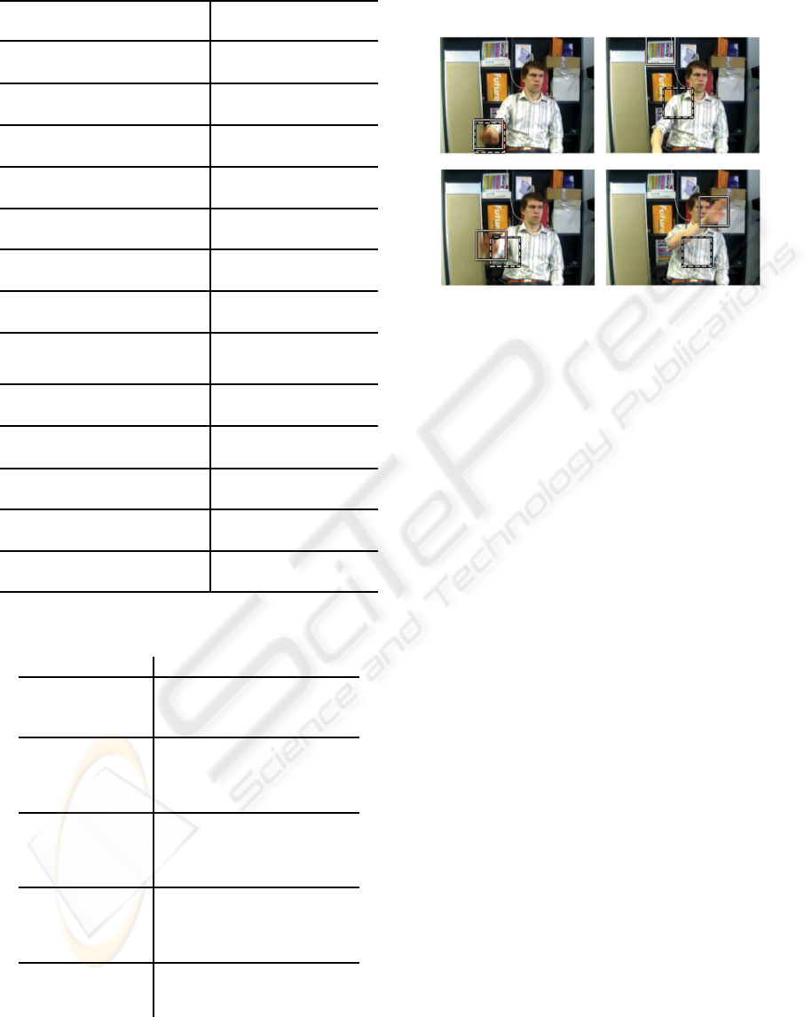
Table 2: Parameters used in the experiments.
N
p
, number of particles 30 30
σ
2
d
, variance of the dy-
namic model
60 60
σ
2
m
, variance of the mea-
surement model
0.1 0.1
R
m
, rectangle size for the
motion cue
61× 61 61× 61
R
c
, rectangle size for the
color cue
11× 11 11× 11
Number of bins in color
histograms
64 64
T
m
, threshold for the mo-
tion cue
15 15
T
ef f
’threshold for resam-
pling
15 15
S
bf
, size of the box filters 91× 91 -
(τ
c
,τ
s
), thresholds for
color model adaptation
(0.5,0.01) -
σ
2
p
, variance of the pro-
posal distribution
70 -
R
e
, the radius for the parti-
cle subset
50 -
k, constant for the velocity
weight
- 0.07
Number of mean shift iter-
ations
- 2
Table 3: Average tracking rates.
FGPF MSEPF
Hand speed
(slow/fast)
0.96 / 0.91 0.89 / 0.67
Background
(sim-
ple/cluttered)
0.93 / 0.95 0.79 / 0.76
User in the
background
(no/yes)
0.97 / 0.93 0.73 / 0.81
Additional per-
son in the back-
ground (no/yes)
0.96 / 0.90 0.80 / 0.73
Average over
all sequences
0.94 0.78
mentarily ambigious. Example frames of the tests are
given in Fig. 3.
Figure 3: Example frames from the test set, where the con-
tinuous and the dashed rectangles mark the estimates of
the FGPF and MSEPF, respectively (frames 207, 209, 212,
230).
5 CONCLUSIONS
In this paper a particle filter approach for hand track-
ing is proposed. The method uses computationally
efficient color based blob features for effective propa-
gation of the particles. Since color cue alone might
be ambiguous, it is augmented with motion cue in
the measurement model. Furthermore, a novel tech-
nique for conditional color model adaptation is pre-
sented, which makes the method invariant to momen-
tarily faults in the location estimate. The experiments
show that the method is able to track the hand in the
presence of complicating factors, such as fast hand
movements and background clutter and movement.
For the future work, the method could be enhanced to
track with a moving camera. At this stage, fast camera
movements would degrade the motion cue and thus
thus make the measurement model less accurate.
REFERENCES
Arulampalam, M. S., Maskell, S., Gordon, N., and Clapp,
T. (2002). A tutorial on particle filters for on-
line nonlinear/non-gaussian bayesian tracking. IEEE
Transactions on Signal Processing, 50(2):174–188.
Bretzner, L., Laptev, I., and Lindeberg, T. (2002). Hand
gesture recognition using multi-scale colour features,
hierarchical models and particle filtering. In Proc. of
FGR, pages 423–428.
Bretzner, L. and Lindeberg, T. (1998). Feature tracking with
automatic selection of spatial scales. Computer Vision
and Image Understanding: CVIU, 71(3):385–392.
A FEATURE GUIDED PARTICLE FILTER FOR ROBUST HAND TRACKING
373

Isard, M. and Blake, A. (1996). Contour tracking by
stochastic propagation of conditional density. In Proc.
of ECCV (1), pages 343–356.
Leonardis, A., Bischof, H., and Pinz, A. (2006). Surf:
Speeded up robust features. In Proc. of ECCV (1),
volume 3951 of Lecture Notes in Computer Science.
Springer.
Lin, J. Y., Wu, Y., and Huang, T. S. (2004). 3d model-based
hand tracking using stochastic direct search method.
In Proc. of FGR, pages 693–698.
Mahmoudi, F. and Parviz, M. (2006). Visual hand track-
ing algorithms. In Geometric Modeling and Imaging–
New Trends, pages 228 – 232.
Pantrigo, J. J., Montemayor, A. S., and Cabido, R. (2005a).
Scatter search particle filter for 2d real-time hands and
face tracking. In Proc. of ICIAP, pages 953–960.
Pantrigo, J. J., Montemayor, A. S., and Sanchez, A.
(2005b). Local search particle filter applied to human-
computer interaction. In Proc. of ISPA, pages 279 –
284.
Pavlovic, V., Sharma, R., and Huang, T. S. (1997). Visual
interpretation of hand gestures for human-computer
interaction: A review. IEEE Transactions on Pattern
Analysis and Machine Intelligence, 19(7):677–695.
P´erez, P., Vermaak, J., and Blake, A. (2004). Data fusion
for visual tracking with particles. Proceedings of the
IEEE (issue on State Estimation), 92:495 – 513.
Rehg, J. M. and Kanade, T. (1993). Digiteyes: Vision-based
human hand tracking. Technical report, Carnegie Mel-
lon University, Pittsburgh, PA, USA.
Shan, C., Wei, Y., Tan, T., and Ojardias, F. (2004). Real
time hand tracking by combining particle filtering and
mean shift. In Proc. of FGR, pages 669–674.
Swain, M. J. and Ballard, D. H. (1991). Color indexing. Int.
J. Comput. Vision, 7(1):11–32.
Viola, P. and Jones, M. (2001). Rapid object detection us-
ing a boosted cascade of simple features. In Proc. of
CVPR.
VISAPP 2008 - International Conference on Computer Vision Theory and Applications
374