CORNER DETECTION ON CURVES

Neeta Nain, Vijay Laxmi and Bhavitavya Bhadviya

Department of Computer Engineering, Malaviya National Institute of Technology Jaipur, JLN Marg, Jaipur-302017, India

Keywords:

Corners, Chain Code, Difference Code, Curvature.

Abstract:

Detection of discontinuity plays an important role in image registration, comparison, segmentation, time se-

quence analysis and object recognition. In this paper we address some aspects of analyzing the content of an

image. A point is classiﬁed as a corner where there are abrupt changes in the curvature of the curve. This paper

presents a new approach for corner detection using ﬁrst order difference of chain codes. Since the proposed

method is based on integer operations it is simple to implement and efﬁcient. Preliminary results are presented

and evaluation with respect to standard corner detectors is done as a benchmark.

1 INTRODUCTION

An edge (Gonzalez and Woods, 2000), by deﬁnition,

is that where drastic change in value from one spot

to the next either in intensity level of an image or in

one’s own eyes takes place. In the digital world, an

edge is a set of connected pixels that lie on the bound-

ary between two regions. Similarly corner detection

(M. Sonka and Boyle, 1993) is identiﬁcation of high

curvature points on planar curves which is referred to

as boundary of an image. A corner can also be de-

ﬁned as the intersection of two edges or, as a point for

which there are two dominant and different edge di-

rections in a local neighborhood. Corners play a dom-

inant role in shape perception by humans. They play

crucial role in decomposing or describing the object.

They are used in scale space theory, image represen-

tation, reconstruction, matching and as preprocessing

phase of outline capturing systems.

This paper proposes a new difference chain encoding

algorithm for corner detection in images. The task

of ﬁnding corners is formulated as a three step pro-

cess. In the ﬁrst step we extract one pixel thick noise-

less boundary by using various morphological opera-

tions. The extracted boundary is chain encoded using

m-connectivity (Gonzalez and Woods, 2000). In the

second step we apply chain smoothing procedures to

remove false corners by suppressing regular intensity

changes. The ﬁnal step calculates difference codes

and then abrupt changes are identiﬁed in them to de-

tect signiﬁcant corners.

2 EXISTING TECHNIQUES

Many corner detection algorithms have been pro-

posed in the literature. Rosenfeld and John-

ston (Rosenfeld and Johnston, 1973) calculate cur-

vature maxima points using k-cosines as corners.

Rosenfeld and Wezka (Rosenfeld and Wezka, 1975)

proposed a modiﬁcation of (Rosenfeld and Johnston,

1973) in which averaged k-cosines were used. Free-

man and Davis (Freeman and Davis, 1977) found

corners at maximum curvature change in which they

move a straight line segment along the curve. An-

gular differences between successive segments was

used to measure local curvature. Beus and Tiu (L.

and Tiu, 1987) algorithm was similar to (Freeman

and Davis, 1977) except they proposed arm cutoff

parameter τ to limit length of straight line. Smith’s

algorithm (Smith and Brady, 1997) involves generat-

ing a circular mask around a given point in an im-

age and then comparing the intensity of neighbor-

ing pixels with that of the center pixel, and repeating

the procedure for each pixel within the image. Har-

ris corner detector (Harris and Stephens, 1988) com-

putes locally averaged moment matrix computed from

the image gradients, and then combines the eigen-

values of the moment matrix to compute a corner

“strength”, of which maximum values indicate the

corner positions. Yung’s (He and Yung, 2004) al-

gorithm starts with extracting the contour of the ob-

ject of interest, and then computes the curvature of

this contour with Gaussian derivative ﬁlters at var-

127

Nain N., Laxmi V. and Bhadviya B. (2008).

CORNER DETECTION ON CURVES.

In Proceedings of the Third International Conference on Computer Graphics Theory and Applications, pages 127-133

DOI: 10.5220/0001094801270133

 SciTePress

ious scales. Local extremes of the product of the

curvatures at different scales are reported as cor-

ners when the value of the product exceeds a thresh-

old. There are various other techniques like wavelets,

Hough transform, neural networks etc using which

corners can be extracted as described in (P and Horng,

1994), (Liu and Srinath, 1990), (Tsai. D.M and Su,

1999), (E.Rosten and Drummong, 2006), (Quddus

and Gabbouj, 2002), (Shen and Wang, 2002), (Sojka,

2002), (Olague and Hernandez, 2005), (Bergevin and

Bubel, 2004), (Bergevin and Bubel, 2003),

3 CORNER DETECTION

It has long been known that information about shape

is conveyed via the changes in the slope of an object’s

boundary.

Algorithm 1 Pseudocode for Calculating -

Corners(S

Require: S

: List of boundary points S, for i = 1, 2, ··· , N

N ! = 0;

Ensure: : Corners of the Curve S

Initialization

l = (N)

{Calculate Edge length parameter}

procedure Corners(S

)

1: Extract Boundary

2: Chain Encode Boundary. Assign BC codes.

3: Calculate Slope.

= tan

−1

(

)

4: Smooth the boundary. Calculate MC codes.

5: Calculate Curvature.

δφ

= φ

i+1

− φ

= mod

(MC

i+1

− MC

+ 8)

6: Avoid false corners.

7: if (MC

= MC

i−n(n=1,2,...,l)

) then

8: false corner at i

position.

9: end if

10: Find true corners.

11: if (P

− P

i−1

> l) then

12: true corners at P

and P

i−1

positions

13: end if{P

- Position of isolated non-zero DC

s.}

14: end procedure

The rate of change of slope is called curvature. The

information content is greatest where curvature is

maximum in a local neighborhood of points. We

present a method of estimating the curvature of a pla-

nar curve, and detecting high-curvature points as cor-

ners on such curves. Digital images are acquired and

processed in a grid format with equal spacing in the

x and y direction. Slope and curvature are difﬁcult

to compute precisely in the digital domain, since the

angle between neighboring pixels is quantized by 45

◦

increments. The basic idea is to estimate the tangent

orientation using edge points that are not adjacent in

the edge list. This allows a larger set of possible tan-

gent orientations. Let P

= (x

, y

) be the coordinates

of edge point i in the edge list. The l−slope is the (an-

gle) direction vector between points that are l edges

apart. The left l−slope is the direction from P

i−l

, and the right l−slope is the direction from P

i+l

. The l−curvature is the difference between the

left and right l−slopes. We identify a corner at the

max(l − curvature). The detailed proposed algo-

rithm is summarized in Algorithm. 1

4 IMPLEMENTATION DETAILS

The proposed technique of corner detection is based

on ﬁnding vertex points on the boundary curve where

two straight line segments meet. The length of the

straight line segment is taken as a parameter l called

pixel neighborhood or edge length. The algorithm

identiﬁes the points where the curvature is highest in

a neighborhood of ±l pixels. The threshold value l,

for our experiments when taken as

l = (BoundaryLength)

(1)

fourth root of the boundary length gives excellent

results. If l is taken less than our threshold then false

corners will be generated as it will capture all the

small curvature changes also. While a larger value

will miss signiﬁcant corners. We deﬁne the lower

bound on l as atleast ≥ 3. This deﬁnes a corner at the

intersection of two edges of atleat 3 pixels length.

4.1 Boundary Extraction

To extract corners we need precise, compact and

continuous in a segment boundary. One-pixel thick

m-connected boundary is extracted using our own

morphological algorithm (Neeta Nain and Agarwal,

2006). One-pixel thick, and m-connectivity avoids

redundancy in chain codes. This boundary is chain-

encoded using 8−way chain encoding (Freeman and

Davis, 1977) method. The boundary chain (BC)

codes are notations for recording the list of edge

points along a contour. The BC code speciﬁes the di-

rection of a contour at each edge point in the edge

list. When 8−way connectivity is used, directions are

quantized into one of eight directions as shown in Fig-

ure 1.

GRAPP 2008 - International Conference on Computer Graphics Theory and Applications

128

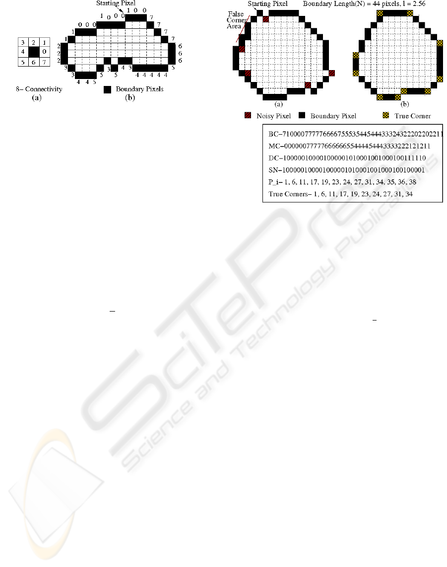
Figure 1: Example: Assignment of Boundary Chain(BC)

codes.

The 360

◦

is divided into eight directions. Each direc-

tion specifying 45

◦

angle from the previous. Thus a

chain code could be generated by starting at the ﬁrst

point in the edge list and going clockwise around the

contour, the direction to the next edge point is speci-

ﬁed using one of the eight chain codes. The direction

is the chain code for the 8−neighbor of the edge. The

chain-code varies from (0..7) in anti-clockwise direc-

tion, where 0 means moving one unit in x direction

making angle 0

◦

with the x- axis, code 1 represents

◦

from x−axis and so on. The BC code thus codes

the slope of the current pixel with the previous.

The slope at pixel i is

= tan

−1

(

) (2)

4.2 Boundary Smoothing

Due to side effects of scan-conversion or aliasing

effects, a straight line in the pixel form is not drawn

as a straight line, but it has some regular changes

also called stair-step effects. The problem gets more

complicated when the radius of curvature is small on

the boundary, or in other words if the slope changes

fast in a small neighborhood of points. Then if we

capture all these slope changes then we generate false

corners. We need to identify only abrupt signiﬁcant

curvature changes on the boundary to detect signiﬁ-

cant corners.

To remove the stray pixels from the boundary in

the neighborhood of ±l pixels, which is equivalent of

convolving with an lxl averaging mask, the BC codes

are further modiﬁed, called Modiﬁed Chain (MC)

codes. The modiﬁcation step smoothens the bound-

ary, removes noise and thus removes false corners

from boundary.

• Remove spurious single pixels from the bound-

ary.

– One pixel breaks in straight line, where there

Figure 2: (a)Original boundary, (b) Single stray pixels re-

moved after smoothing step.

is only one isolated pixel above the break. A

V made by a set of pixels.

– One pixel thick diagonal line with one extra

pixel in 4-neighborhood of any of the pixel of

this diagonal line. A L made by a set of pixels.

A run of l constant BC codes represents an

edge of length l, with slope =

BC. If between

two edges of length atleast l, there are three

stray pixels making an angle 45

◦

then we

smooth them. Table 1 shows some of the

modiﬁcation for BC codes to smooth the

stray pixels. For pixel i if the left l−slope

depicted by BC

i−l

to BC

, and the right l−slope

depicted by BC

to BC

i+l

is same and there

are three continous pixels with different

we modify them as shown in Table 1.

For example, refer Figure 2(a), its BC code

=(710000777776666755535445444333243222

02202211). After removing the spurious single

pixels from the boundary MC code = 00000077

77766666655444454443333222121211. Fig-

ure 2(b) shows the result of the smoothing step.

• This smoothing step is done only when the ap-

plication requires the convex hull or the bound-

ing extent of the ﬁgure and its corners.

Align stray single pixels along the dominant

slope in a 3x3 neighborhood. Where dominant

slope is max (count(BC

i±n(n=1,2,3)

))

For current pixel position i

– If BC

i+n(n=1,2)

= BC

i−n(n=1,2)

AND BC

i±n

then BC

= BC

i+1

– If (BC

i−n(n=1,2)

= BC

i+1

AND 6= BC

) OR

CORNER DETECTION ON CURVES

129

Table 1: Code modiﬁcations for smoothing stray pixels

from the boundary.

Current BC Codes Modiﬁed MC Codes

(0, 7, 1) / (0, 1, 7) (0, 0)

(2, 3, 1) / (2, 1, 3) (2, 2)

(4, 5, 3) / (4, 3, 5) (4, 4)

(6, 5, 7) / (6, 7, 5) (6, 6)

(1, 2, 0) / (1, 0, 2) (1, 1)

(3, 4, 2) / (3, 2, 4) (3, 3)

(5, 6, 4) / (5, 4, 6) (5, 5)

(7, 0, 6) / (7, 6, 0) (7, 7)

(2, 0, 2) (2, 1)

(4, 6, 4) (4, 4)

(5, 3, 5) (5, 4)

(BC

i+n(n=1,2)

= BC

i−1

AND 6= BC

) then

= BC

i+1

(or BC

= BC

i−1

– If (BC

i−n(n=1,2)

= BC

i+2

AND BC

6= BC

i+2

)

OR (BC

i+n(n=1,2)

= BC

i−2

AND BC

6= BC

i−2

)

then BC

= BC

i+2

(or BC

= BC

i−2

This step modiﬁes all the spurious codes

on the curve and aligns the stray pixels

along the dominant slope of the line. For

example, after this step the false corner

area marked in Figure 2(b) will get smooth

along 45

◦

. The MC code after this step

=000000777776666665544444444333322222

1111, depicting the convex hull of the ﬁgure

smoothing all the small edges in the direction

of the dominant slope.

4.3 Avoid False Corners

Let for pixel position i, If MC

6= MC

i−1

, then

it is called the ﬁrst occurrence of MC code.

If the ﬁrst occurrence MC

= MC

i±n(n=1,2,...,l)

then the i

position is not a corner.

For our example, N(BoundaryLength) =

44; l = 2.56, and the MC code =

0000007777766666655444454443333222121211,

then its ﬁrst occurrence MC code positions are

(1, 6, 11, 17, 19, 23, 24, 27, 31, 34, 35, 36, 37, 39). The

MC code at (35, 36, 37, 39, 40)

position already ex-

ists in previous or next codes within a neighborhood

of l = 2.56, and thus are positions of false corners

and not marked.

4.4 Find True Corners

The curvature of the curve is obtained by calculating

the ﬁrst derivative of the MC code. The ﬁrst deriva-

tive of the MC code, obtained by ﬁrst difference of

the MC code, is a rotation-invariant boundary descrip-

tion. The curvature at current pixel i is δφ

= φ

i+1

−φ

which is calculated as

= mod

(MC

i+1

− MC

+ 8) (3)

The ﬁrst order difference code (DC) on the MC

codes represents this curvature or turning angle from

the previous point. If DC

i±l

= 0 it is an edge. Let

denotes the position of isolated non-zero DC

in a sequence of zero DC

s. If P

− P

i−1

≥ l (the

difference between consecutive positions of isolated

non zero DC’s). Then there are true corners at P

and P

i−1

positions. For our example, the MC code =

(0000007777766666655444454443333222121211),

its DC = (00000700007000007070001700700070071

7170)(DC code is calculated by treating the MC code

as a circular chain). The non-zero DC positions P

are (1, 6, 11, 17, 19, 23, 24, 27, 31, 34, 35, 36, 37, 39).

The difference between non zero DC positions

≥ l(= 2.57), at (1, 6, 11, 17, 19, 23, 24, 27, 31, 34)

positions hence they are identiﬁed as true corners as

shown in Figure 2(b).

5 TEST RESULTS

A corner detection algorithm must be tested on a va-

riety of shapes for its proper evaluation. Our test

images include most variety of variations in curva-

ture, corner sharpness and noise/irregularities along

the boundary curves. Such variations are expected in

real life images. Our corner detector gives single, lo-

calized and accurate response to corners. Compari-

son is also done with two popular algorithms namely

Harris (Harris and Stephens, 1988) and Yung (He and

Yung, 2004) with their default parameters. Table 2

and Figures 3, 4 and 5 shows the results. Both Harris

and Yung miss true corners on small curvature curves.

Our corner detector gives excellent results even in the

presence of noise like Gaussian, Poisson, and Speckle

etc., while both Harris (Harris and Stephens, 1988)

and Yung (He and Yung, 2004) are not invariant to

noise. They eliminate some true corners and also in-

troduce false corners due to noise. Noisy test images

are generated by adding Gaussian noise with 0 mean

and 0.01 variance as default values. Poisson noise is

generated from the image data following Poisson dis-

tribution. Salt-and-Pepper noise is generated with a

noise density of 0.02, and Speckle noise is a multi-

plicative uniformly distributed noise with 0 mean and

variance 0.04. Our algorithm is invariant to Gaussian,

Poisson and Speckle noise and extracts all true cor-

ners as shown in Figure 6. Though it generates some

GRAPP 2008 - International Conference on Computer Graphics Theory and Applications

130

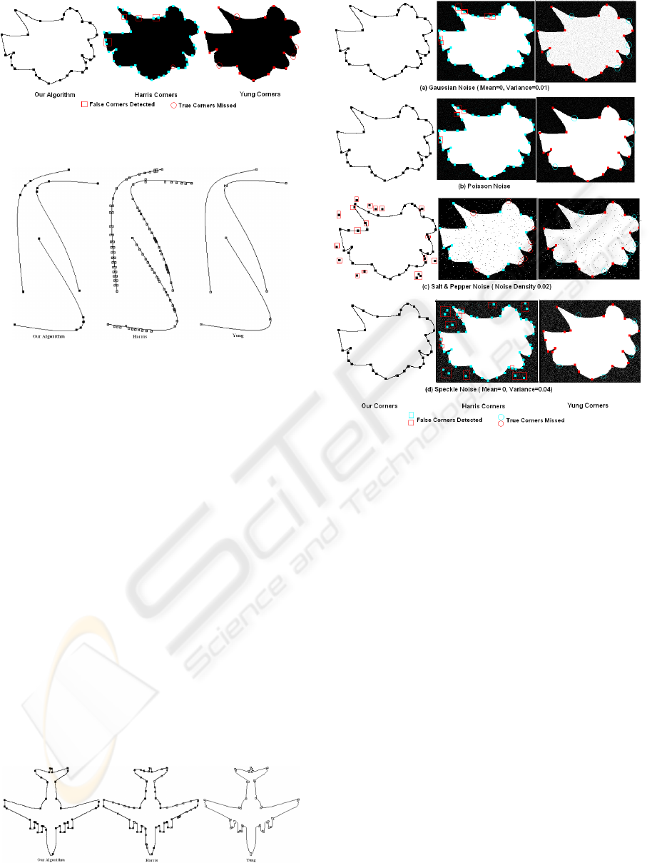
Figure 3: Test image with sudden changes in curvature.

Figure 4: Test image with smooth changes in curvature.

false corners in Salt-and-Pepper noisy images. We

can overcome this problem by eroding the small im-

age segments introduced by noise.

6 AFFINE TRANSFORMATION

INVARIANCE

Any transformation effects like translation, rotation,

shearing and minor size variations should not effect

corner detection results. Our algorithm is afﬁne trans-

formation invariant.

1. Translation Invariance: Corners are calculated

on the ﬁrst order differences of the chain codes.

The ﬁrst difference in the chain codes makes the

boundary translation invariant as they represent

the turning angles from the previous point.

2. Scale Invariance: To expand or to contract a chain

by a speciﬁed scale factor, one must appropri-

ately scale each chain link and then re quantize.

Figure 5: Test image with straight lines and curves.

Figure 6: Corners extracted on noisy images (a) Gaussian

Noise, (b) Poisson Noise, Salt-n-Pepper Noise, (d) Speckle

Noise.

In down sampling, a number of links may merge

into one, and in up-sampling one link may cause

a string of many links to be generated. The gen-

eration of these new links is most easily handled

by using Bresenham scan conversion technique.

Compared to up sampling, down sampling is ro-

bust to aliasing effects. We down sample the

boundary to a constant size before chain coding.

This re sampling makes the corner detector scale

invariant.

3. Orientation Invariance: The derivative of the MC

code, also called DC code, obtained by using ﬁrst

difference, is a rotation-invariant boundary de-

scription. Further We align the boundary with

minimum angle with the x− axis. This is done

by circularly shifting the DC

s and starting with

the ﬁrst difference of smallest magnitude. Circu-

lar shift makes the boundary rotation invariant and

the corners extracted on this boundary will be ro-

tation invariant.

The test results of our transformation invariant cor-

ner detection algorithm on the standard test image is

shown in Figure 7.

CORNER DETECTION ON CURVES

131

Figure 7: Transformation invariance of corner extractor(a)

Original (b) Rotated by 90

◦

, (c) Scaled 50% (d) Scaled 50%

and Rotated 180

◦

7 CONCLUSIONS

In this paper we proposed a novel simple, efﬁcient and

transformation invariant method for corner detection

which uses only integer arithmetic for approximation

of curvature on curve boundary. The algorithm de-

pends on only one parameter l. The parameter l, can

be assigned a constant value as per personal prefer-

ence of neighborhood, and it is also adaptive to the

length of the boundary curve. Experimental results

show that l taken as fourth root of boundary length is

sufﬁcient for extracting good corners. The parameter

l is therefore both local and global in nature. Com-

parative study on various noiseless and noisy images

has been done. Finally, the comparison between the

proposed approach and other corner detectors show

that our approach is more competitive with respect to

Harris (Harris and Stephens, 1988) and Yung (He and

Yung, 2004) under similarity and afﬁne transforms.

Moreover, a number of experiments also illustrate that

our corner detection has more robustness to noise.

Table 2: Comparison of corner detectors on Figures 3, 4

and 5.

Corner Results Figure

Detector

Yung True Corners Missed on 3

Curved Edges

Harris Poor True Corners even

on Signiﬁcant Curvature

Change.False Corners

even on Small Curvature

Change 3, 4, 5

Our All True Corners, No

Algorithm False Corners. Better

Approximation of

Curvature Change 3, 4, 5

Corners extracted from this technique could be used

in various shape analysis (Neeta Nain and Agarwal,

2007), size measurement and boundary reconstruc-

tion applications. From the extracted corners we can

easily reconstruct the boundary by ﬁtting straight line

segments between corners. This can be used as the

convex hull or an approximation to the object’s shape.

REFERENCES

Bergevin, R. and Bubel, A. (2003). Object-level structured

contour map extraction. Computer Vision and Image

Understanding, 91(3):302–334.

Bergevin, R. and Bubel, A. (2004). Detection and charac-

terization of junctions in a 2d image. Computer Vision

and Image Understanding, 93(3):288–309.

E.Rosten and Drummong, T. (May 2006). Machine learning

for high-speed corner detection. European Conference

on Computer Vision, Citeseer.

Freeman, H. and Davis, L. S. (1977). In A Corner Finding

Algorithm for Chain Coded Curves, volume 26, pages

297–303. IEEE Transaction in Computing.

Gonzalez, R. C. and Woods, R. E. (2000). Digital Image

Processing. Addison Wesley Longman, 2nd edition.

Harris, C. and Stephens, M. (1988). In A Combined Cor-

ner and Edge Detector, volume 23, pages 189–192.

Proceedings of 4th Alvey Vision Conference, Manch-

ester.

He, X. C. and Yung, N. H. C. (2004). Curvature scale

space corner detector with adaptive threshold and dy-

namic region of support. In ICPR ’04: Proceedings

of the Pattern Recognition, 17th International Confer-

ence on (ICPR’04) Volume 2, pages 791–794, Wash-

ington, DC, USA. IEEE Computer Society.

L., B. H. and Tiu, S. S. (1987). In An Improved Corner

Detection Based on Chain Coded Plane Curves, vol-

ume 20, pages 291–296. Pattern Recognition Letters.

Liu, H. and Srinath, M. (1990). In Corner Detection from

Chain Code, volume 23, pages 51–68. Pattern Recog-

nition Letters.

M. Sonka, V. H. and Boyle, R. (1993). Image Processing

Analysis and Machine Vision. Chapman and Hall, 2nd

edition.

Neeta Nain, Vijay Laxmi, A. K. J. and Agarwal, R. (2006).

In Morphological Edge Detection and Corner De-

tection Algorithm Using Chain-Encoding, volume II,

pages 520–525. The 2006 International Conference on

Image Processing, Computer Vision, Pattern Recog-

nition, Las Vegas, Nevada, USA.

Neeta Nain, Vijay Laxmi, M. K. and Agarwal, D. (2007).

Transformation invariant robust shape analysis. In The

2007 International Conference on Image Processing,

Computer Vision and Pattern recognition, pages 275–

281, Nevada, USA. CSREA Press.

Olague, G. and Hernandez, B. (2005). A new accurate and

ﬂexible model based multi-corner detector for mea-

surement and recognition. Pattern Recognition Let-

ters, 26(1):27–41.

P, C. S. and Horng, J. H. (1994). In Corner Point De-

tection Using Nest Moving Average, volume 27(11),

pages 1533–1537. Pattern Recognition Letters.

Quddus, A. and Gabbouj, M. (2002). Wavelet-based cor-

ner detection technique using optimal scale. Pattern

Recogn. Lett., 23(1-3):215–220.

GRAPP 2008 - International Conference on Computer Graphics Theory and Applications

132

Rosenfeld, A. and Johnston, E. (1973). In Angle Detec-

tion on Digital Curves, volume C-22, pages 875–878.

IEEE Transactions on Computers.

Rosenfeld, A. and Wezka, J. S. (1975). In An Improved

Method of Angle Detection on Digital Curves, volume

C-24, pages 940–941. IEEE Transactions on Comput-

ers.

Shen, F. and Wang, H. (2002). Corner detection based on

modiﬁed hough transform. Pattern Recognition Let-

ters, 23(8):1039–1049.

Smith, S. M. and Brady, J. M. (1997). Susana new approach

to low level image processing. volume 23, pages 45–

78, Hingham, MA, USA. Kluwer Academic Publish-

ers.

Sojka, E. (2002). A new algorithm for detecting corners

in digital images. In SCCG ’02: Proceedings of the

18th spring conference on Computer graphics, pages

55–62, New York, NY, USA. ACM Press.

Tsai. D.M, H. H. and Su, H. J. (1999). In Boundary Based

Corner Detection Using Neural Networks, volume 20,

pages 31–40. Pattern Recognition Letters.

CORNER DETECTION ON CURVES

133