HYBRID MATCHING OF UNCALIBRATED OMNIDIRECTIONAL

AND PERSPECTIVE IMAGES

Luis Puig, J. J. Guerrero

DIIS-I3A, University of Zaragoza, Zaragoza, Spain

Peter Sturm

INRIA Rh

one-Alpes, Montbonnot, France

Keywords:

Computer vision, matching omnidirectional images, hybrid epipolar geometry.

Abstract:

This work presents an automatic hybrid matching of central catadioptric and perspective images. It is based

on the hybrid epipolar geometry. The goal is to obtain correspondences between an omnidirectional image

and a conventional perspective image taken from different points of view. Mixing both kind of images has

multiple applications, since an omnidirectional image captures many information and perspective images are

the simplest way of acquisition. Scale invariant features with a simple unwrapping are considered to help

the initial putative matching. Then a robust technique gives an estimation of the hybrid fundamental matrix,

to avoid outliers. Experimental results with real image pairs show the feasibility of that hybrid and difﬁcult

matching problem.

1 INTRODUCTION

Recently, a number of catadioptric camera designs

have appeared. The catadioptric cameras combine

lenses and mirrors to capture a wide, often panoramic

ﬁeld of view. It is advantageous to capture a wide

ﬁeld of view for the following reasons. First, a wide

ﬁeld of view eases the search for correspondences as

the corresponding points do not disappear from the

images so often. Second, a wide ﬁeld of view helps

to stabilize egomotion estimation algorithms, so that

the rotation of the camera can be easily distinguished

from its translation. Last but not least, almost com-

plete reconstructions of a surrounding scene can be

obtained from two panoramic images (Svoboda and

Pajdla, 2002).

A hybrid image matching is a system capable of

establish a relation between two or more images com-

ing from different camera types. The combination of

omnidirectional and perspective images is important

in the sense of that a single omnidirectional image

contains more complete description of the object or

place it represents than a perspective image thanks to

its wide ﬁeld of view and its ability to unfold objects.

In general if we want to establish a relation be-

tween two or more views obtained from different

cameras, they must have a common representation

where they can be compared. We face this problem

when we want to match omnidirectional images with

perspective ones. Few authors have dealt with this

problem and they followed different strategies. In

(Menem and Pajdla, 2004) Pl

ucker coordinates are

used to map ℘

into ℘

where lines and conics are

represented in 6-vectors and a geometrical relation

can be established. A change of feature space is in-

troduced in (Chen and Yang, 2005). The perspec-

tive image is partitioned into patches and then each

patch is registered in the Haar feature space. These

approaches have a major drawback, they require in-

formation about the geometry of the particular mirror

used to get the images, which in most cases is not

available. Besides they perform hard transformations

over the image.

Another approach to deal with this problem is to

establish a geometric relation between the images.

Sturm (Sturm, 2002) develops this type of relation be-

tween multiple views of a static scene, where these

views are obtained from para-catadioptric and per-

spective cameras.

We propose to explore a way to overcome these

drawbacks avoiding the use of the so complex geo-

metry of the mirror and the formulation of a geomet-

125

Puig L., J. Guerrero J. and Sturm P. (2008).

HYBRID MATCHING OF UNCALIBRATED OMNIDIRECTIONAL AND PERSPECTIVE IMAGES.

In Proceedings of the Fifth International Conference on Informatics in Control, Automation and Robotics - RA, pages 125-128

DOI: 10.5220/0001494901250128

 SciTePress

ric model. We present an automatic hybrid matching

approach with uncalibrated images using the hybrid

epipolar geometry to establish a relation between om-

nidirectional and perspective images.

2 HYBRID IMAGE MATCHING

USING EPIPOLAR GEOMETRY

To deal with the problem of the robust hybrid match-

ing a common strategy is to establish a geometrical re-

lation between the views of the 3D scene. We have se-

lected a strategy that does not require any information

about the mirror. A geometrical approach which en-

capsulates the projective geometry between two views

is used. Epipolar geometry (EG) is the intrinsic pro-

jective geometry between two views. It is indepen-

dent of the scene structure, and only depends on the

cameras’ internal parameters and relative pose (Hart-

ley and Zisserman, 2000). This approach needs pairs

of putative corresponding points between the views.

In this work we use the SIFT descriptor (Lowe, 2004).

Sturm proposes a hybrid epipolar geometry, where

a point in the perspective image is mapped to its corre-

sponding epipolar conic in the omnidirectional image.

Recently Barreto and Daniliidis (Barreto and Dani-

ilidis, 2006) have exposed a more general scheme

where they compare the mixture of central cameras,

including pin-hole, hyperbolic and parabolic mirrors

in catadioptric systems and perspective cameras with

radial distortion.

The fundamental matrix F encapsulates the epipo-

lar geometry. The dimension of this matrix depends

on the image types we want to match. In the hybrid

case we have two options, a 4 × 3 matrix in the case of

para-catadioptric and perspective cameras or 6 × 3 in

the case of hyperbolic mirror and perspective cameras

in a catadioptric system. In (Barreto and Daniilidis,

2006) for this last case a 6 × 6 matrix is considered,

which can result in a very difﬁcult corresponding es-

timation problem.

2.1 EG with Perspective and

Catadioptric Cameras

In general the relation between omnidirectional and

perspective images with the fundamental matrix can

be established by

= 0 (1)

subscripts p and c denote perspective and catadioptric

respectively.

From Eq.1 with known corresponding points bet-

ween the two images, we can derive the hybrid fun-

damental matrix. Points in the perspective image are

deﬁned in common homogeneous coordinates. Points

in the omnidirectional image are deﬁned depending

on the shape of the epipolar conic. The general repre-

sentation for any shape of epipolar conic is a 6-vector.

A special case where the shape of the conic is a circle

the coordinate vector has four elements. These repre-

sentations are called the “lifted coordinates” of a point

in the omnidirectional image.

In the hybrid epipolar geometry points in the

perspective image are mapped to its corresponding

epipolar conic in the omnidirectional image. Conics

can be represented in homogeneous coordinates as the

product

c = 0, where

represents the lifted coor-

dinates of the omniﬁrectional point q. In this work

we have two representations for this point, one of

them is the general homogeneus form of a conic, a

6-vector

q = (q

, q

)

. The other

one constraints the shape of the conic to be a circle

q = (q

+ q

, q

)

. These representations

are called the “lifted coordinates” of the omnidirec-

tional point q.

If the point in the omnidirectional image is repre-

sented with a 6-vector lifted coordinates

q, the fun-

damental matrix is 6 × 3 (F63) in such a way that

c ∼ F

. When the 4-vector lifted coordinates is

used the fundamental matrix is 4 × 3 and the conic

(circle) is obtained by the same product c ∼ F

2.2 Computation of the Hybrid

Fundamental Matrix

The algorithm used to compute the fundamental ma-

trix is similar to the 8-point algorithm (Hartley and

Zisserman, 2000) for the purely perspective case, with

the difference that the points in the omnidirectional

images are given in lifted coordinates.

The automatic computation of the fundamental

matrix is summarized as follows:

1. Initial Matching. Scale invariant features are ex-

tracted in each image and matched based on their

intensity neighborhood.

2. RANSAC Robust Estimation. Repeat for n sam-

ples, where n is determined adaptively:

(a) Select a random sample of k corresponding

points, where k depends on what model we are

using (if F43, k = 11 or if F63, k = 17)

. Com-

pute the hybrid fundamental matrix F

as de-

scribed above.

Matrices are up to scale, so we need the number of ele-

ments of the matrix minus one corresponding points.

ICINCO 2008 - International Conference on Informatics in Control, Automation and Robotics

126

(b) Compute the distance d for each putative cor-

respondence, d is the geometric distance from

a point to its corresponding epipolar conic

(Sturm and Gargallo, 2007).

by the number of correspondences for

which d < t pixels.

Choose the F

with the largest number of inliers.

The F

is used to eliminate outliers which are

those point correspondences for which d > t.

3 HYBRID EG EXPERIMENTS

In this section we present experiments performed with

real images obtained from two different omnidirec-

tional cameras. The ﬁrst one is a model composed by

an unknown shape mirror and a perspective camera.

The second one is composed by a hyperbolic mirror

and a perspective camera.

The purpose of this experiment is to show the

performance of this approach to compute the hybrid

epipolar geometry in real images. We use 40 manu-

ally selected corresponding points to compute it. In

order to measure the performance of F we calculate

the geometric error from each point to its correspond-

ing epipolar conic. Fig.1(a) shows the epipolar con-

ics computed with the F43 matrix using the unknown

shape mirror. Fig. 1(b) shows the epipolar conics

computed with the F63 matrix using the hyperbolic

mirror. The mean of distances from the points to

their corresponding epipolar conics are 2.07 pixels

and 0.95 pixels respectively.

(a) Experiment with the unknown shape mirror using F43.

(b) Experiment with the hyperbolic using F63.

Figure 1: Experiments with real images using both mirrors

and both hybrid fundamental matrices.

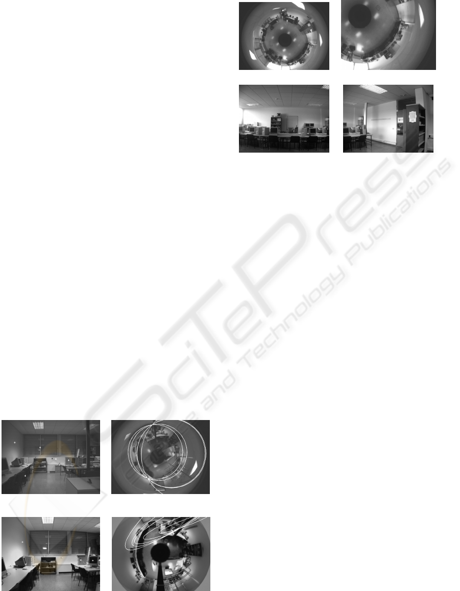
(a) (b)

Figure 2: Set of images used to test the automatic approach.

(a) Omnidirectional image. (b) An image cut from (a). (c)

Perspective1 image. (d) Perspective2 image.

4 AUTOMATIC MATCHING

In this section we present some experiments perform-

ing automatically the matching between an omnidi-

rectional and a perspective image. There exist ap-

proaches matching automatically omnidirectional im-

ages using scale invariant features (Murillo et al.,

2007) which demonstrate a good performance, but it

does not work with hybrid matching. An easy way to

transform an omnidirectional image into a common

environment with the perspective one is to unwrap the

omnidirectional image, which consists in a mapping

from Cartesian to polar coordinates.

The initial matching between the perspective and

the unwrapped omnidirectional image has a consid-

erable amount of inliers but also a majority of out-

liers. This scenario is ideal to use a technique like

RANSAC where we have a set of possible correspon-

dences of points useful to compute the hybrid epipolar

geometry.

One omnidirectional image, a part of it and two

perspective images, all of them uncalibrated, are used

to perform the following experiment. We use the al-

gorithm explained in section 2.2. Table 1 summarizes

the results of this experiments giving the quantity of

inliers and outliers in the initial and the robust match-

ing. For example, in Experiment 1 we use images

Fig.2(a) and Fig.2(c). The initial matching gives a

35% of inliers. After applying the robust estimation

we obtain a 80% of inliers. Notice that just 2 inliers

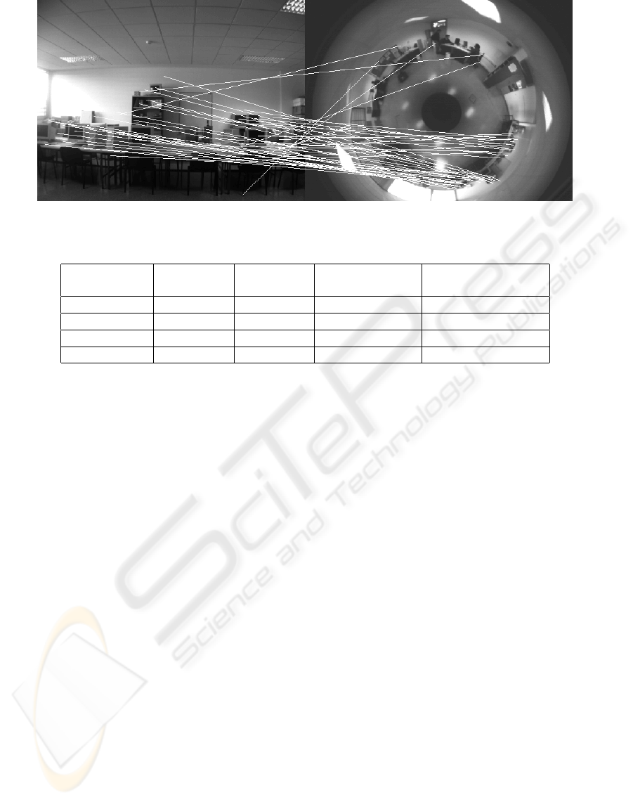
have been eliminated. Fig. 3 shows the ﬁnal matches.

The results show that the epipolar geometry elim-

inates most of the outliers. For practical reasons in

the estimation problem, we use the F43, the simplest

model of the hybrid epipolar fundamental matrix.

HYBRID MATCHING OF UNCALIBRATED OMNIDIRECTIONAL AND PERSPECTIVE IMAGES

127

Figure 3: Matching between omnidirectional and perspective image using the unwrapping and the hybrid EG as a tool.

Table 1: Numerical results of the matches using the set of images.

Omni SIFT Persp SIFT

Initial Matches Robust EG matches

(inliers/outliers) (inliers/outliers)

Experiment 1 636 941 37/70 35/9

Experiment 2 636 1229 19/36 16/11

Experiment 3 246 941 36/11 34/4

Experiment 4 246 1229 20/14 16/6

5 CONCLUSIONS

In this work we have presented an automatic wide-

baseline hybrid matching system using uncalibrated

cameras. We have performed experiments using real

images with different mirrors and two different ways

to compute the hybrid fundamental matrix, a 6-vector

generic model and a reduced 4-vector model. The

last one has demonstrated be useful in order to require

fewer iterations to compute a robust fundamental ma-

trix and having equal or even better performance than

the 6-vector approach. We also prove that an easy

polar transformation can be a useful tool to perform a

basic matching between omnidirectional and perspec-

tive images. Finally the robust automatic matching

proved its efﬁciency to match an omnidirectional im-

age and a perspective image, both uncalibrated.

ACKNOWLEDGEMENTS

This work was supported by project NERO DPI2006

07928 and DGA(CONSI+D)/CAI.

REFERENCES

Barreto, J. P. and Daniilidis, K. (2006). Epipolar geome-

try of central projection systems using veronese maps.

In CVPR ’06: Proceedings of the 2006 IEEE Com-

puter Society Conference on Computer Vision and

Pattern Recognition, pages 1258–1265, Washington,

DC, USA. IEEE Computer Society.

Chen, D. and Yang, J. (2005). Image registration with

uncalibrated cameras in hybrid vision systems. In

WACV/MOTION, pages 427–432.

Hartley, R. I. and Zisserman, A. (2000). Multiple View Ge-

ometry in Computer Vision. Cambridge University

Press, ISBN: 0521623049.

Lowe, D. (2004). Distinctive image features from scale-

invariant keypoints. In International Journal of Com-

puter Vision, volume 20, pages 91–110.

Menem, M. and Pajdla, T. (2004). Constraints on perspec-

tive images and circular panoramas. In Andreas, H.,

Barman, S., and Ellis, T., editors, BMVC 2004: Pro-

ceedings of the 15th British Machine Vision Confer-

ence, London, UK. BMVA, British Machine Vision

Association.

Murillo, A. C., Guerrero, J. J., and Sag

ues, C. (2007). Surf

features for efﬁcient robot localization with omnidi-

rectional images. In 2007 IEEE International Confer-

ence on Robotics and Automatio, Roma.

Sturm, P. (2002). Mixing catadioptric and perspective cam-

eras. In Workshop on Omnidirectional Vision, Copen-

hagen, Denmark, pages 37–44.

Sturm, P. and Gargallo, P. (2007). Conic ﬁtting using the

geometric distance. In Proceedings of the Asian Con-

ference on Computer Vision, Tokyo, Japan. Springer.

Svoboda, T. and Pajdla, T. (2002). Epipolar geometry for

central catadioptric cameras. Int. J. Comput. Vision,

49(1):23–37.

ICINCO 2008 - International Conference on Informatics in Control, Automation and Robotics

128