STRUCTURE, SCALE-SPACE AND DECAY OF OTSU’S
THRESHOLD IN IMAGES FOR FOREGROUND/BACKGROUND
DISCRIMINATION
R. Walia and R. Jarvis
Department of ECSE, Monash University, Clayton, Victoria-3028, Australia
Keywords: Scale-Space Theory, Pattern Recognition in Image Understanding, Segmentation and Grouping.
Abstract: A method for gauging the appropriate scale for foreground-background discrimination in Scale-Space
theory is presented. Otsu’s Threshold (OT) is a statistical parameter generated from the first two moments
of a histogram of a signal / image. In the current work a set of OT is derived from histograms of derivatives
of image having Scale-Space representation. This set of OT, when plotted against corresponding scale,
generates a Threshold Graph (TG). The TG undergoes an exponential decay, in the absence of foreground
and exhibits inflection(s) in the presence of foreground. It is demonstrated, using synthetic and natural
images, that the maxima of inflection indicate the scale and threshold (OT) appropriate to interface edges.
The edges identified by thresholding at scale and threshold given by inflection of OT correspond to
foreground-background interface edges. The histogram inherently imbeds the TG with underlying image
signal parameters like background intensity range, pattern frequency, foreground-background intensity
gradient, foreground size etc, making the method adaptable and deployable for unsupervised machine vision
applications. Commutative, separable and symmetric properties of the Scale-Space representation of an
image and its derivatives are preserved and computationally efficient implementations are available.
1 INTRODUCTION
Scale-Space theory for image processing constitutes
an important component of early vision (Lindberg,
1994). However, any pragmatic implementation of
Scale-Space theory requires ascertaining the
appropriate scale (Lindberg, 1994). This is a trivial
task for well posed problems like in medical
imaging where abundant apriori information (size,
position, color, shape etc) is accessible. However,
deciding the appropriate scale by machine vision is
ill-posed for (a) images without access to apriori
information e.g. in exploratory robotics wherein the
environment changes continuously and
unexpectedly, (b) evolutionary images like dynamic
textures, anomaly detection in granite, wood, or in
mining where apriori information is rendered
redundant owing to evolution with each frame or
image.
In addition to the problem of identifying the
appropriate scale, there is often a requirement for
identifying the foreground within an image. In this
paper a novel method is proposed to identify both
the appropriate scale as well as the foreground in the
image at that scale by using the same parameter. The
parameter used is Otsu Threshold (Otsu, 1979) for
segmenting the image. This paper has following
contributions:
(a) Surveys contemporary methods for scale
identification and establishes the need to
identify scale relevant to the whole image
rather than local entities like pixels, edges,
blobs etc.
(b) Proposes a novel method wherein scale is
determined in response to global
characteristics of image as opposed to local
properties of images.
(c) Validates the method on a range of image
parameters on synthetic and natural images
and backgrounds.
2 SCALE IDENTIFICATION
Pioneering work by (Witkin, 1981), (Koenderink,
1984) and (Lindberg, 1994) has lead to Scale-Space
120
Walia R. and Jarvis R. (2009).
STRUCTURE, SCALE-SPACE AND DECAY OF OTSU’S THRESHOLD IN IMAGES FOR FOREGROUND/BACKGROUND DISCRIMINATION.
In Proceedings of the Fourth International Conference on Computer Vision Theory and Applications, pages 120-128
DOI: 10.5220/0001755101200128
Copyright
c
 SciTePress

theory. The basic tenant of this theory is to imbed a
signal (image) into one-parameter of derived signals
(images), the Scale-Space where the parameter
denoted scale describes the image at the current
level of scale. The image L(x,y) when expressed as a
function of scale (t) is represented as L(x,y; t) and is
obtained by convolving the image L(x,y) with a
Gaussian kernel G(x,y;t) centered at point P(x,y) and
having a variance t
t)y;G(x, y)L(x, t)y;L(x,
⊗
=
where
(1)
t
yx
e
t
tyxG
2
22
2
1
);,(
+
−
=
π
(2)
2.1 Scale Identification Methods
(Lindberg, 1994) describes the problem of
establishing an appropriate scale in the absence of
apriori as intractable. Although models emulating
mammalian vision take cognizance of the need to
establish an appropriate scale they do not
exclusively address this need, but rather skirt
around it by using large scales (Malik. and
Perorna, 1990) or contextual scales (Ren et al,
2006). (Lindberg, 1994) addresses scale
identification in two different ways.
The first one involves a 4-Dimensional
structure composed of a scale-space-blob
generated from data driven structure detection in
images. This structure is tracked over multi scales
with the hypothesis that prominent structures
persist across scales. Blobs are derived at different
scales using monotonic gradients from local
extrema and are then analyzed for their effective
scale range using blob-descriptors like volume,
contrast and area, and blob-events like
annihilation, creation, merging and splitting.
In the second approach by Lindberg (Lindberg,
1994) utilizes the principle of non enhancement of
extrema as applicable to Gaussian differential
operators. A normalized (with scale) and
consequently scale invariant Gaussian derivative
operator is traced for maxima over scales. The
scale corresponding to the maxima is heuristically
hypothesized to coincide with the characteristic
length of corresponding structure in image data.
For a rigorous mathematical treatment, the reader
is referred to chapter 13 of (Lindberg, 1994).
2.2 Drawbacks of Scale Identification
Methods
These two methods are based on qualitative
assumptions and mathematical derivations thereof.
However these approaches have a “top-down”
approach in tracing the entities (blob / edge of
interest), wherein the entities are detected at a finer
scale and their behavior traced to a coarser level. This
approach has three drawbacks.
The first one arises from the use of local properties
in the initial identification of entity which, in the case
of blobs, is seeding originating from a blob event and,
in the case of Gaussian derivative operator, is the edge
maxima. Both these entities are dependent on local
spatial properties like the intensity and nearness to
another entity which often give rise to spurious
structures. In the case of the Gaussian derivative
operator, all the edges (including noise) are
guaranteed a maximum (
Lindberg, 1994) over some
scale; hence the problem of appropriate scale
identification still persists. To address this problem a
ranking mechanism grades the entities based on
properties of entities like contrast, life, spatial spread,
volume etc across the scales. The ranking mechanism
is unreliable as the local properties like the geometry
of entity will influence both the Scale-Space evolution
as well as the properties over scale. For example
response to a Gaussian derivative of a curved edge
will vary from that of a straight edge and, without
apriori information on the kind of edge being
detected, the response will be unreliable and in fact
can often lead to a choice of improper derivative
function.
The second drawback arises from the restricted
spatial scope of local extrema. Fig 1 (a) shows a 1
dimensional signal (termed original) comprising of
local maxima in the vicinity of global minima of the
signal. The original signal is convolved with 3
Gaussian kernels as shown in Fig 1(b). The standard
deviations of the 3 kernels coincide with the spatial
spread of local extrema (Gauss 1), neighborhood of
local extrema (Gauss 2) and the global neighborhood
of local extrema (Gauss 3). The results of convolving
with Gauss 1, Gauss 2 and Gauss 3 are also shown in
Fig 1(a) by Result 1, Result 2 and Result 3,
respectively. The evolution of local maxima is shown
inside the dotted rectangle of 1(a). This evolution
indicates that:
(a) Local extrema violates the principle of non-
enhancement of extrema, as the intensity of
local extrema is first reduced and then
increased with increasing scale. This violation
is not due to scale increment but due to
STRUCTURE, SCALE-SPACE AND DECAY OF OTSU'S THRESHOLD IN IMAGES FOR
FOREGROUND/BACKGROUND DISCRIMINATION
121

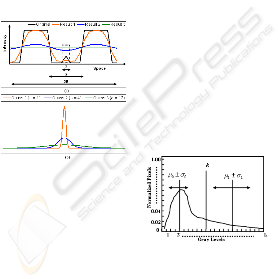
consideration of local extrema in isolation
from global neighborhood.
(b) Evolution of local maxima can have valid but
conflicting classification depending on the
scale. E.g. based on Result 1 the local extrema
can be hypothesized as local maxima and
based on Result 2 as global minima. There
are two solutions to ascertain the appropriate
classification. The first one (inapplicable in
current context) is to have apriori information
on the appropriate scale and the second is to
have a global analysis rather than a local.
Figure 1: (a) 1D signal with spatial spreads of local
extrema, local neighbourhood and global neighborhood
and the results of convolution with Gaussian kernels at b.
(b) Gaussian kernels corresponding to spatial spread of
local extrema {Gauss 1, σ = (3-1)/2}, local neighbourhood
{Gauss 2, σ = (9-1)/2}, global neighbourhood {Gauss 3, σ
= (25-1)/2}.
The third drawback arises from a plausibly
flawed hypothesis due to minimal representation of
image. The methods (Lindberg, 1994) to identify
appropriate scale omit the evolution of non-extrema
neighborhood with scale. This neighborhood is
quantitatively significant as locating even the first
cut (zeroth scale) extrema involves discarding 8
neighboring pixels. Increasing the scale also
increases the discarded neighborhood due to non-
enhancement property. Hence the important
structures are generated from a hypothesis based on
a minimal representation of the image.
2.3 Proposed Method
In the current paper a “bottom-up” approach will be
presented. In view of the drawbacks of establishing
the optimum scale using local methods, the authors
contend, that since incremental scales affect the
extrema as well as the accompanying neighborhood,
the impact of increasing Gaussian scales needs to be
observed globally (entire image or a section of image
that extends beyond the spatial extent of local feature)
and not locally. To facilitate a global observation of
the Scale-Space representation of entire image, it is
desirable to have an image feature which can:
(a) Encompass the entire image.
(b) Embed underlying image signal features.
(c) Exist at all scales.
(d) Quantitatively identify the appropriate scale.
(e) Segregate important structures in the image.
Usage of Otsu’s threshold as an image parameter
for scale determination addresses the above
requirements. Otsu’s threshold is calculated at
increasing scales from magnitude of Sobel edge of
image, for identifying appropriate scale. Gray level
Image Histograms derived from Scale-Space
representation of images satisfies requirements (a) to
(c). Otsu Threshold (Otsu, 1979) bifurcates an image
thereby addressing requirement (e). Section 3
illustrates compliance with requirement (d) by
creation of peaks when Otsu’s Threshold is plotted
against increasing scale. These peaks can be uniquely
located and quantitatively defined.
Figure 2: Visual representation of Otsu’s Threshold.
Otsu’s threshold (Otsu, 1979) is statistically
generated from a normalized histogram for L gray
levels in an image. Each gray level represents the
pixels at that gray level as a percentage of total
pixels in the image. This normalized histogram is
bifurcated into two hypothetical classes C0 and C1
at a hypothetical threshold k. Hypothetical threshold
VISAPP 2009 - International Conference on Computer Vision Theory and Applications
122

(k), Mean and Standard Deviations of classes
)(
000
σ
μ
±C
and
)(
111
σ
μ
±
C
are shown in Fig 2.
The maximum of Between Class Variance (BCV)
determines the appropriate threshold. BCV is
defined as:
Where
(3)
(0
th
Order cumulative Moment for C
0
)
(4)
(0
th
Order cumulative Moment for C
1
)
(5)
(Mean Gray Level for the Image)
(6)
(Mean Gray Level for C
0
)
(7)
(Mean Gra
y
Level for C
1
)
(8)
(1
st
Order cumulative Moment upto level k
of histo
g
ram)
(9)
Normalised probability at level i ;
n
i
: number of pixels at level i;
N : Total pixels in image
(10)
While the Otsu’s algorithm segregates the image, it
does not classify foreground and background of
segregated image in the absence of apriori
information. Different segregation methods would
be required for separating a darker foreground as
compared to a brighter foreground for the same
background. Usage of magnitude of Sobel edges in a
image leads to uniformity of classification as the
problem of distinguishing a foreground from
background is transformed into one wherein
interface (foreground-background) edges are
required to be segregated from non-interface edges.
This method assumes that non-interface edges
originate from homogenous textures (Foreground or
Background) whereas interface edges arise from
heterogeneous textures (Foreground and
Background). It is therefore justifiably assumed that
interface edges exhibit greater magnitude of gradient
as compared to foreground-foreground or
background-background edges, thus generating a
group of edges amenable to segregation. Usage of
first order derivative (sobel edges of an image)
preserves the scale-space properties associated with
zeroth order signal (original image) (Lindberg,
1994).
This approach addresses all the issues associated
with scale identification listed in section 2.2 as the
histograms are generated from magnitude of edges of
entire image. The important structures are then
segregated by bifurcation of the histograms. Since
these structures originate from global calculations
rather than local, they are relatively impervious to the
local properties. The structures so obtained originate
w.r.t. background and consequently do not require
relative grading algorithms
.
3 ALGORITHM & PROPERTIES:
THRESHOLD GRAPH (TG)
Otsu’s threshold is calculated for first derivative of
the Gaussian smoothed image for each scale to
generate a Gaussian Smoothed Derivative Image
(GSDI). Specifically, magnitudes of Sobel’s edges
are used as a first derivative of Image. The
algorithm for plotting the Threshold (Steps 1, 2),
identifying the optimum scale (step 3) and
identifying important structure in the GSDI (Step 5)
is outlined in Algorithm 1.
Algorithm 1:
1. Convolve the image with Gaussian Kernel of
increasing scale. For each scale :
a. Calculate the histogram from Magnitude
of Sobel edges.
b. Calculate OT from the histogram.
c. Record OT against the scale.
2. Plot OT against the scales.
3. Identify the scale at which local maxima
exists in the TG. For all the results presented
in this paper the local maxima was identified
2
11
2
00
)()(
TTB
μμωμμω
ν
−+−=
∑
=
=
k
i
i
p
0
0
ω
0
1
1
1 ωω −==
∑
+=
L
ki
i
p
∑
=
=
L
i
iT
ip
0
μ
0
0
ω
γ
μ
K
=
1
1
ω
γ
μ
μ
KT
−
=
∑
=
=
k
i
iK
ip
0
γ
Nnp
ii
/=
STRUCTURE, SCALE-SPACE AND DECAY OF OTSU'S THRESHOLD IN IMAGES FOR
FOREGROUND/BACKGROUND DISCRIMINATION
123

by the maximum of difference operator (
∇
).
Difference operator is defined as
)1()()(
2
−−=∇
<<=
kTkTk
Lk
(11)
Where
L is the maximum scale under consideration
T (k) represents the Otsu’s threshold at scale k
The optimum scale k
*
is given by the
maximum positive difference operator:
)](max[)(
*
2
kk
Lk
∇=∇
<<=
(12)
If
0)( >∇ k
4. Absence of any positive Difference Operator
indicates absence of a foreground entity.
5. If an optimum scale with corresponding OT is
identified, the image is segmented by
Thresholding the GSDI with OT.
Note 1: Steps 3, 4 in algorithm 1 demonstrate that
the process of detecting maxima and scale can be
automated. The steps are not exhaustive and
replaceable by other methods (beyond the scope
of current paper) to detect maxima in signals.
3.1 Background Intensity Variation
The tiles in the Fig 3 are from images (Syn 1, 2, 3, 4,
5 and 6) of dimensions 640X480 with the intensities
as listed in Table 1. The gradient magnitude between
foreground and background of three sets of
complimentary images (Syn 1, 4; 2, 5; 3, 6) is
identical although the gradient direction of FG and
BG is reverse. The TGs of complimentary sets of
synthetic GSDIs are shown in Fig 4. Each
complimentary pair has identical TG which leads to
following two deductions:
(a) OT decay is exponential and proportional to
the magnitude of gradient.
(b) Decay is independent of gradient direction.
Table 1: Intensities of Syn 1 to 6.
Image:
(Syn)
1
2 3 4 5 6
Foreground
Intensity
0 0 0 255 255 255
Background
Intensity
85 170 255 170 85 0
Figure 3: Tiles of Synthetic Images. (a) Syn 1 (b) Syn 2
(c) Syn 3 (d) Syn 4 (e) Syn 5 (f) Syn 6.
0
20
40
60
80
100
120
1.1
1.4
1.7
2
2.
3
2.
6
2.
9
3
.2
3
.5
3
.8
4.1
4.4
4.7
5
5.3
5.6
5.9
Scale
Otsu Threshold
Syn 1 Syn 2 Syn 3
Syn 4 Syn 5 Syn 6
Figure 4: TG of Pairs Syn (1,4), (2,5), (3,6).
3.2 Background Intensity Variation
Tiles and TG from synthetic images Syn 10, 11, and
12 are shown in Fig 5. In each image pattern
wherein the intensity is same but the frequency of
background is varied. TG indicates that the OT
decays with minor variations in decay rate due to
background frequency.
Figure 5: Top Row(Left to Right) – Tiles of Synthetic
Images Syn 10,11 and 12. Bottom Row – TG of Syn 10,11
and 12.
VISAPP 2009 - International Conference on Computer Vision Theory and Applications
124

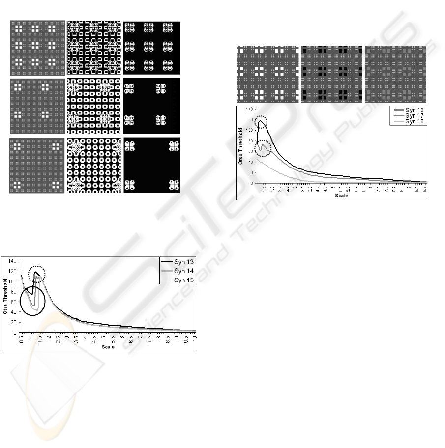
3.3 Foreground Frequency Variation
In synthetic Images Syn 13, 14, 15 the background
pattern comprises of square clusters of intensity 170
against a backdrop of intensity 85. The foreground
comprises of cluster of four squares of intensity 255
and a size of 4 pixels each. These foreground
clusters are separated by distance of 8, 16 and 24 for
Syn 13, 14 and 15 respectively as illustrated by tiles
in first column of Figure 6. The TG due to
Algorithm 1 is shown in Figure 7.
Figure 6: Top, Middle and Bottom Row: Images Syn 13,
14 and 15. First, Second and Third Column: Tiles of
Synthetic Image, Thresholded Images at Lower Inflection
point and Upper Inflection point.
Figure 7: TG of Syn 13, 14 and 15.
The results of thresholding the image with the
Otsu’s threshold at the lower and upper points of
inflection are shown in second and third column of
Fig 6. It is observed that the appropriate scale
respect to the background of the image is given by
the upper point of inflection. Column 3 of Fig 6
shows that the thresholded images at upper points of
inflection give the important structure in the image
with respect to the background. This quantitative
event (maxima) enables TG to:
(a) Detect scale and threshold appropriate to a
image.
(b) Identify the important structures (in this case
represented by edges) in the image.
A slight shift in the local maxima is observed
with decrease of the foreground frequency, which
can be attributed to attrition in the percentage of
pixels contributing to histogram bin at the
background-foreground interface. Nevertheless the
ability of the TG to adapt to the internal structure of
the image background is illustrated.
3.4 Foreground Intensity Variation
Figure 8: Top Row(Left to Right)- Tiles of Syn 16, 17 and
18. Bottom Row: TG of Syn 16, 17 and 18.
Images Syn 16, 17 and 18 shown in Fig 8 have
the same pattern as the image Syn 13, however the
foreground intensity is set to 255, 0 and 127
respectively. Since the background intensity varies
between 85 and 170, three scenarios are:
i. Foreground intensity>Background range (Syn 16)
ii. Foreground intensity<Background range (Syn 17)
iii. Foreground intensity is within the Background
range (Syn 18)
The TGs are depicted in Fig 8. Where the
foreground intensity is beyond the background
intensity range, inflection exists in the TG. However
when the foreground intensity range is confined to
the range exhibited by the background (TG for Syn
18) the inflection does not occur; hence the
important structures are not detected. Absence of
inflection can be attributed to similar interface
derivatives as the non-interface derivatives. It is a
unique case and does not occur frequently,
especially in natural textures e.g. detecting a grass
hopper in grass. Natural textures like pebbles, sand,
water, hay, grass, vegetation, wood, and even
manmade textures like rugs, carpets usually have
STRUCTURE, SCALE-SPACE AND DECAY OF OTSU'S THRESHOLD IN IMAGES FOR
FOREGROUND/BACKGROUND DISCRIMINATION
125

background chromaticity which when projected
onto gray scale has a narrow range. Consequently
the foreground object’s intensity exists outside the
background image intensity range.
3.5 Foreground Size Variation
Three sets of synthetic images and their TG are
shown in Fig 9 to 15 where Set 1 corresponds to
Fig 9 (Syn 19 to 27) and Fig 12 (TG of Syn 19 to
27); Set 2 corresponds to Fig 10 (Syn 28 to 36) and
Fig 13 (TG of Syn 28 to 36); Set 3 corresponds to
Fig 11 (Syn 37 to 45) and Fig 14 (TG of Syn 37 to
45);. Each set of Synthetic images contains a
rectangular foreground of varying sizes having
area 0.01, 0.04, 0.09, 0.16, 0.25, 0.36, 0.49, 0.64
times that of the synthetic image. Reduced images
are shown owing to paucity of space; however the
background patterns are shown in top row second
column of Fig 13, 15, 17 respectively for sets 1, 2
and 3. The thresholded GSDI at the points of
inflection of TG for all the 3 sets are shown in:
(a) In 3 cases of background only i.e. Syn 19,
28 and 37 represented by black lines in
Fig 14, 16 and 18 there is only decay of
the TG without any inflection. Remaining
TG of synthetic images however undergo
an inflection even on introduction of
foreground of area 1 % of total image
area.
Figure 9: Top Row (Left to Right) Shrunk Images Syn 19 to 27. Bottom Row - Results. Bottom Row 1
st
Column:
Background Pattern for Syn 19 to 27.
Figure 10: Top Row (Left to Right) Shrunk Images Syn 28 to 36. Bottom Row - Results. Bottom Row 1st Column:
Background Pattern for Syn 28 to 36.
Figure 11: Top Row (Left to Right) Shrunk Images Syn 37 to 45. Bottom Row - Results. Bottom Row 1st Column:
Background Pattern for Syn 37 to 45.
Figure 12: TG of Syn 19 to 27. Figure 13: TG of Syn 28 to 36. Figure 14: TG of Syn 37 to 45.
VISAPP 2009 - International Conference on Computer Vision Theory and Applications
126

(b) Intra set points of inflection for all 3 sets
reveal a decreasing trend (dotted ellipses)
with increase of foreground area. The
intra-set trend of decrease of non-
interface class mean (Δμ
0
) being more
than increase of interface class mean
(Δμ
1
) results in decrease of threshold (k)
due to equation 13 (Lin,2003)
2/)(
10
μ
μ
+=k (13)
(c) Inter set points of inflection exhibit an
increasing range of inflection values with
respect to scale as shown by the dotted
ellipses in Fig 12, 13 and 14. Background
frequency is decreasing from set 1 to 2 to
3, hence threshold’s (k) sensitivity
increases to term (μ
1
) in equation 13,
resulting in increased range of inflection
values.
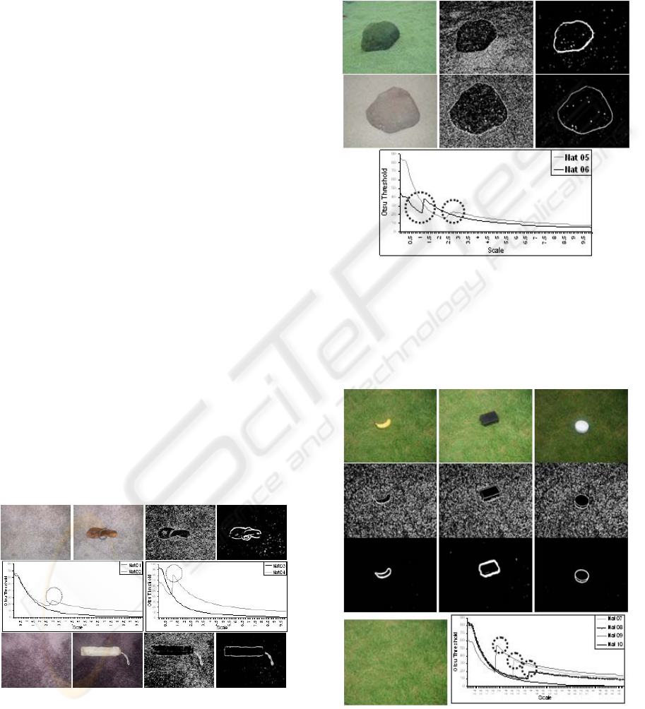
3.6 Natural Images
Natural scenes comprise of a host of image signal
distortion factors like ambient light, shadows, 2-D
representation of 3-D space, occlusion and
projection of 3-D chromaticity onto grayscale.
There are image acquisition problems arising out
of camera position, resolution and digital
representation which aggravate the difficulty in
estimation of appropriate scale. In addition a
singular appropriate-scale as applicable to entire
image will not exist in images wherein the
coarseness of back ground pattern changes across
the scene. In spite of inherent problems in locating
Figure 15: Top Row (Left to Right)-Natural Images
Nat01 Nat 02, Thresholded Nat02 at lower and upper
points of inflection. Middle Row-TG of Nat01, 02, 03
and 04. Bottom Row (Left to Right)-Natural Images
Nat03 Nat04, Thresholded Nat04 at lower and upper
points of inflection.
the appropriate scale in natural images, OT is fairly
robust in detecting background-foreground
interface. Figures 15 to 18 present result of
applying OT to various backgrounds both in the
presence and absence of foreground.
Figure 16: Top Row (Left to Right)-Natural Image
Nat05 Original, and Thresholded at lower inflection
point, and upper inflection point. Middle Row: Natural
Image Nat06 Original, Thresholded at lower inflection
point and upper inflection point. Bottom Row: TG of
Nat05 and Nat06.
Figure 17: 1
st
Row (Left to Right)-Natural Image Nat07,
Nat08, Nat09. 2
nd
Row: Nat07, Nat08 and Nat09
Thresholded at lower inflection points. 3
rd
Row: Nat07,
Nat08 and Nat09 Thresholded at upper inflection points.
Bottom Row: Nat10 and TG of Nat07, 08, 09 and 10.
STRUCTURE, SCALE-SPACE AND DECAY OF OTSU'S THRESHOLD IN IMAGES FOR
FOREGROUND/BACKGROUND DISCRIMINATION
127

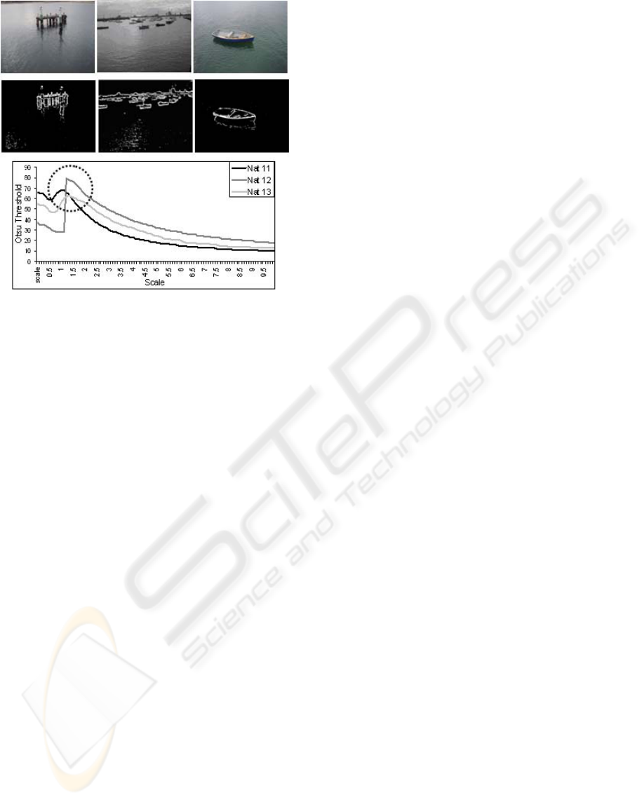
Figure 18: Row 1-Nat11, Nat12, Nat13, Row 4-TG of
Nat11, 12, 13. Column 1 and 2 – Original and
Thresholded Image (at upper point of inflection).
4 CONCLUSIONS
A novel “bottom-up” concept has been presented
for identifying the important structures and
appropriate scale using Scale-Space properties of
images. The method is unsupervised and addresses
the intractability of scale identification. Synthetic
images have demonstrated the adaptability of the
Threshold Graph to variations in the image. The
results have also been demonstrated on natural and
manmade textures.
This paper has dealt with the structures in
reference to the whole image, but the same
approach can be spatially reduced to find structures
in regions of the images. Scale at points of
inflection can also be used as a parameter in a
variety of region based algorithms. Noise in results
can be eliminated by one or combination of
following
(a) Utilizing a scale higher than that of the
inflection, as the important edges will persevere
across scales.
(b) Hysteresis thresholding across scales.
(c) Sequentially thresholding the interface
edges identified by Otsu’s threshold.
Future research would be on the pre-processing
and post-processing required for extending the
applicability of the TG. Another interesting
application for which TG can be utilized is in
establishing equivalence between space and time
for dynamic textures exhibited by fluids, based on
the assumption that the deformation of fluids in
space and time is similar.
REFERENCES
Lindberg, T. Scale Space Theory in Computer Vision.
Kluwer academic Publishers, Netherlands,. 1994.
Otsu. N. A threshold selection method from gray-level
histograms. IEEE Transactions on Systems, Man
and Cybernetics, SMC-9:62-66, Jan 1979.
Witkin A. Scale-Space Filtering. Proc. Int. Joint Conf on
artificial Intel, Karlsruhe, Germany, 1019-1021,
1981.
Koenderink. J.J. The Structure of Images. Biological
Cybernetics, vol 50, pp. 363-370,1984.
Malik. J. and Perorna. P. Preattentive texture
discrimination with early vision mechanisms. J. Opt
Soc Am A.,7(5): 923-32,1990.
Ren. X, Fowlkes. C and Malik. J. Figure/Ground
Assignment in Natural Images. LNCS, Volume
3952-ECCV2006, pp 614-627, July 2006.
Lin. K.C. Fast image thresholding by finding the zero(s)
of the first derivative of between-class variance.
Machine Vision and Applications (2003) 13: pp 254-
262.
VISAPP 2009 - International Conference on Computer Vision Theory and Applications
128