ROAD INTERPRETATION FOR DRIVER ASSISTANCE BASED ON

AN EARLY COGNITIVE VISION SYSTEM

Emre Bas¸eski

†

, Lars Baunegaard With Jensen

†

, Nicolas Pugeault

†

, Florian Pilz

Karl Pauwels

‡

, Marc M. Van Hulle

‡

, Florentin W

org

otter

∗

and Norbert Kr

uger

†

The Mærsk Mc-Kinney Møller Institute, Univeristy of Southern Denmark, Odense, Denmark

Department for Media Technology, Aalborg University Copenhagen, Copenhagen, Denmark

‡

Laboratorium voor Neuro- en Psychofysiologie, K.U.Leuven, Belgium

∗

Bernstein Center for Computational Neuroscience, University of G

ottingen, G

ottingen, Germany

Keywords:

Large scale maps, Lane detection, Independently moving objects.

Abstract:

In this work, we address the problem of road interpretation for driver assistance based on an early cognitive

vision system. The structure of a road and the relevant trafﬁc are interpreted in terms of ego-motion estimation

of the car, independently moving objects on the road, lane markers and large scale maps of the road. We make

use of temporal and spatial disambiguation mechanisms to increase the reliability of visually extracted 2D and

3D information. This information is then used to interpret the layout of the road by using lane markers that are

detected via Bayesian reasoning. We also estimate the ego-motion of the car which is used to create large scale

maps of the road and also to detect independently moving objects. Sample results for the presented algorithms

are shown on a stereo image sequence, that has been collected from a structured road.

1 INTRODUCTION

A driver assistance system or an autonomous vehicle

requires a road interpretation in terms of layout of the

road and the relevant trafﬁc. The main elements of

such a road interpretation can be summarized as a)

the lanes of the road, b) the rigid body motion esti-

mation of the car, c) independently moving objects

(IMOs) on the road and d) large scale maps of the

road. In this article, we present algorithms for all the

sub-problems, based on information provided by an

early cognitive vision system (Kr

uger et al., 2004).

We make use of visually extracted data from a stereo

camera system. A hierarchical visual representation is

created to interpret the whole scene in 2D and 3D. We

then make use of temporal and spatial disambiguation

mechanisms to increase the reliability of the extracted

information. The layout of the street is calculated

from the disambiguated data by using Bayesian rea-

soning. The ego-motion estimation of the car is done

within the same representation and this information is

used to create large scale semantic maps of the road as

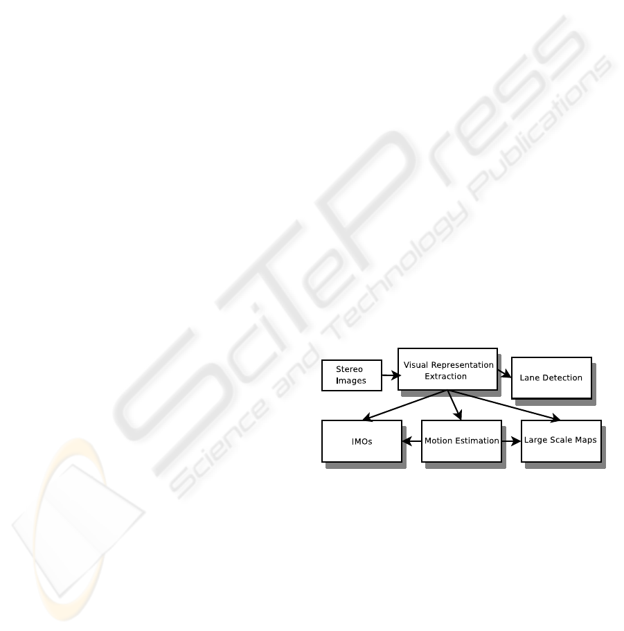
well as to detect and interpret the IMOs. In Figure 1,

Figure 1: General overview of the system.

the general overview of the extraction process of the

whole interpretation is presented. Note that, all sub-

parts of the system use the same visual representation

based on an early cognitive vision system.

Lane detection and parametrization, in particu-

lar in 3D, is acknowledged to be a difﬁcult prob-

lem on which a lot of research is performed currently

(Bertozzi and Broggi, 1998; Wang et al., 2004; Mc-

Call and Trivedi, 2004). The difﬁculty comes from

a) the extraction of relevant information in far dis-

tances, b) the extraction of 3D information (in partic-

ular in hilly environments), and c) poor image qual-

ity and highly varying lightning conditions (leading,

496

Ba¸seski E., Baunegaard With Jensen L., Pugeault N., Pilz F., Pauwels K., M. Van Hulle M., Wörgötter F. and Krüger N. (2009).

ROAD INTERPRETATION FOR DRIVER ASSISTANCE BASED ON AN EARLY COGNITIVE VISION SYSTEM.

In Proceedings of the Fourth International Conference on Computer Vision Theory and Applications, pages 496-505

DOI: 10.5220/0001796104960505

 SciTePress

Figure 2: Satellite image of the road from which the reference stereo image sequence has been collected.Note that, the driving

direction is from left to right.

e.g., to cast shadows). For 2D and 3D lane inter-

pretation, there are already systems build into cars

(see (Bertozzi et al., 2000) for an overview) which

however only give information at the current position

while for driving future positions and other parame-

ters (such as curvature) are of importance.

Moreover, besides the interpretation of the lane

itself, the motion and shape of independently mov-

ing objects (IMOs) need to be integrated into such

lane descriptions which, especially in 3D, is a very

hard problem since not only the scene needs to be

segmented into IMOs and non-IMOs but also the 6D

motion vector as well as the shape of the IMOs need

to be computed based on only the small image areas

the IMOs appear in. Current approaches towards this

problem typically integrate object detection, tracking,

and geometrical constraints (see e.g., (Leibe et al.,

2007)). Such methods crucially rely on object de-

tection, which is very difﬁcult for small or distant

objects. Our method on the other hand, can pro-

vide the required higher precision by integrating mul-

tiple dense cues, namely dense disparity, dense op-

tical ﬂow, and self-motion derived from this optical

ﬂow. The methods used to obtain these cues (see e.g.,

(Pauwels and Van Hulle, 2008)) are robust to typi-

cal nuisance factors observed in real-world video se-

quences recorded by moving observers, such as con-

trast changes, unstable camera motion, and ambigu-

ous camera motion conﬁgurations.

The ego-motion estimation of the car is not only

crucial for extraction of IMOs but also for creating 3D

maps of the road. These maps are similar to SLAM

(see e.g., (Lemaire et al., 2007)) applications and they

can be used to generate global driving events like the

car’s trajectory. Also, this kind of maps are important

in terms of learning the behavior of the driver to use

for driver assistance.

The extraction of such complex information is

time-consuming. In our approach, real-time is not

thought to be achieved through simpliﬁcation of pro-

cesses via specializing on sub-aspects, but by parallel

processing on hardware. In this context, we have de-

veloped a hybrid architecture similar to (Jensen et al.,

2008), consisting of different FPGAs as well as a

coarse parallel computer.

The results explained in this article are also to be

seen as a ﬁrst step towards reasonable benchmark-

ing in the driver assistance domain. It has been dis-

cussed in, e.g., (Hermann and Klette, 2008; Klette,

2008), that the currently used benchmarks in the com-

puter vision community are very suitable to evalu-

ate stereo and optic ﬂow algorithms in controlled en-

vironments but are not very suitable to evaluate al-

gorithms in the context of driver assistance systems

since the demands are very different from the exist-

ing benchmarks. On the other hand, Klette et al. is

in the process of establishing appropriate standard se-

quences of realistic complexity that are published on

’http://www.citr.auckland.ac.nz/6D/’ where also the

sequence on which we show results in this paper is

available. In this way, we think this paper fosters the

process of comparing results on realistic databases for

driver assistance.

The rest of the article is organized as follows: In

Section 2, the early cognitive vision system that has

been used for this work is explained brieﬂy. The al-

gorithms for the sub-parts of the road interpretation

motion estimation, large scale maps, lane detection

and independently moving objects are presented in

Sections 3, 5, 6 and 7 respectively while the disam-

biguation process is discussed in Section 4. Note

that, for evaluation of the presented algorithms, sam-

ple results are demonstrated on a reference sequence

of stereo images collected from a driving on the road

that is shown in Figure 2. We conclude with a discus-

sion on these sample results in Section 8.

2 VISUAL REPRESENTATIONS

In this work we use a representation of visual in-

formation based on local descriptors called ‘primi-

tives’ (Kr

uger et al., 2004). Primitives are extracted

sparsely along image contours, and form a feature

vector aggregating multiple visual modalities such as

position, orientation, phase, color and optical ﬂow.

This results in the following feature vector:

π = (x, θ,φ,(c

),f) (1)

Image contours are therefore encoded as collinear

strings of primitives. Because of that, collinear and

ROAD INTERPRETATION FOR DRIVER ASSISTANCE BASED ON AN EARLY COGNITIVE VISION SYSTEM

497

similar primitives are denoted as ‘groups’ in the fol-

lowing. These are matched across two stereo views,

and pairs of corresponding 2D-primitives afford the

reconstruction of a 3-dimensional equivalent called

3D–primitive, and encoded by the vector:

Π = (X, Θ,Φ,(C

)) (2)

Moreover, if two primitives are collinear and simi-

lar in an image, and their correspondence in the sec-

ond image are also, then the two reconstructed 3D-

primitives are grouped. Extracted 2D and 3D primi-

tives for a sample stereo image pair are illustrated in

Figure 3.

3 MOTION ESTIMATION

In the driving context, rigid body motion is prevalent.

In our work, the motion is estimated using a combi-

nation of SIFT (Lowe, 2004) and primitives features

(see Section 2) in a RANSAC (Fischler and Bolles,

1981) scheme. SIFT features are scale invariant fea-

tures that have been very successfully applied to a

variety of problems during the recent years. They

afford to be matched very robustly across different

views, and provide a robust basis to the motion esti-

mation scheme. On the other hand, their localisation

is imprecise. The primitives provide very accurate

(sub–pixel) localisation, but are less readily matched.

Moreover, because the primitives are local contour

descriptors they only provide motion information in

the direction normal to the contour’s local orienta-

tion. This is an issue in a driving scenario where the

main features, the road lines, are mostly radially dis-

tributed from the car’s heading direction. This means

that most of the extracted primitives yield very lit-

tle information about translation in the z axis. This

limitation can be remediated by using a mixture of

features for motion estimation. In this work, we in-

tegrated both features in a RANSAC scheme, where

SIFT are used for the initial estimation, and the con-

sensus are formed using a combination of SIFT and

primitives. For the motion estimation algorithm we

chose (Rosenhahn et al., 2001), since in addition of

being able to deal with different visual entities, it does

optimization using a twist formulation which directly

acts on the parameters of rigid-body motions.

The results presented in this chapter contain mo-

tion estimation results for feature sets consisting of

primitives, SIFT and a combination of both. Results

are shown in Figure 4, where each column depicts

the translational and rotational motion components

for one type of feature set.

The ﬁrst row in Figure 4 depicting the transla-

tion, the z-axis corresponds to the car’s forward mo-

tion. Here, results show that SIFT and the combina-

tion of SIFT and primitives provide much more sta-

ble results. However outliers still remain, caused by

speed-bumps, potholes etc. These results in blurred

images as on frame 720-730 caused by a bump on the

bridge, making matching and motion estimation a dif-

ﬁcult task.

The second row in Figure 4 depicts the rota-

tional component where y-axis corresponds to rota-

tion caused by steering input. The rotation results for

the y-axis using SIFT and the combination of SIFT

and primitives nicely corresponds to the satellite im-

age presented in Figure 2. This correspondence be-

tween sub-parts of the road and sub-parts of the mo-

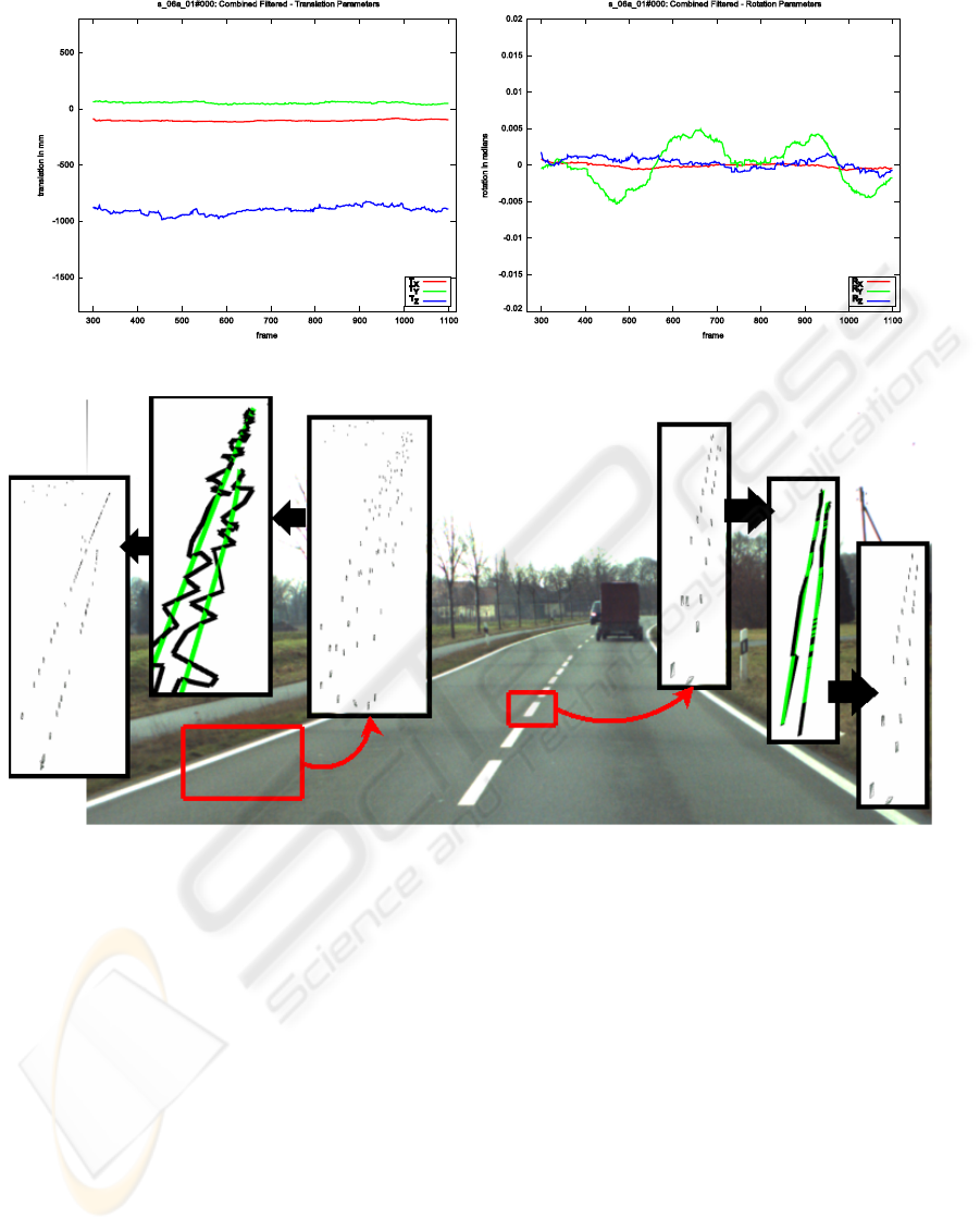
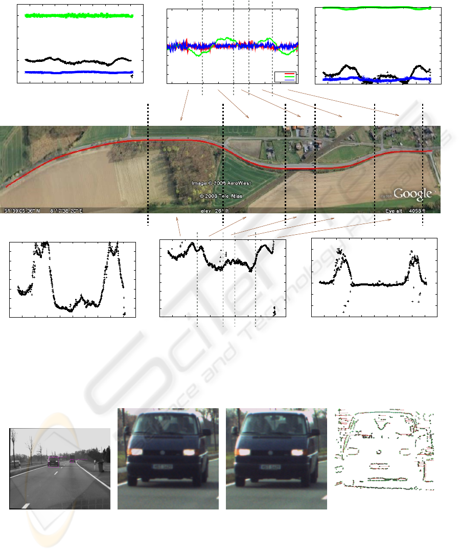
tion estimation plot is shown in Figure 10 (b). Fig-

ure 5 shows translation and rotation obtained after ap-

plying a Bootstrap Filter (Gordon et al., 1993) (us-

ing 1000 particles). This results in the elimination of

the largest variations in the estimated motions and to

more stable results.

4 DISAMBIGUATION

Since 3D-primitives are reconstructed from stereo,

they suffer from noise and ambiguity. Noise is due to

the relatively large distance to the objects observed,

and the relatively small baseline of the stereo rig (33

cm). The ambiguity rises from the matching prob-

lem: despite their multi-modal aspect, the primitives

only describe a very small area of the image, and

similar primitives abound in an image. The epipo-

lar constraint limits the matching problem, yet it is

unavoidable that some ambiguous stereo matches oc-

cur (Faugeras, 1993). We introduce two means of

disambiguation making use of temporal (Section 4.1)

and spatial (Section 4.2) regularities employed by the

early cognitive vision system.

4.1 Temporal Disambiguation

A ﬁrst means of disambiguation is to track prim-

itives over time. We perform this tracking in the

3D space, to reduce the likelihood of false positives.

This involves resolving three problems: ﬁrst, estimat-

ing the motion; second, matching predicted and ob-

served primitives; and third, accumulating represen-

tation over time.

Using the 3D-primitives extracted at a time t and

the computed ego–motion of the car between times

t and t + δt, we can generate predictions for the vi-

sual representation at time t + δt. Moreover, conﬂict-

ing hypotheses (reconstructed from ambiguous stereo

matches) will generate distinct predictions. In most

VISAPP 2009 - International Conference on Computer Vision Theory and Applications

498

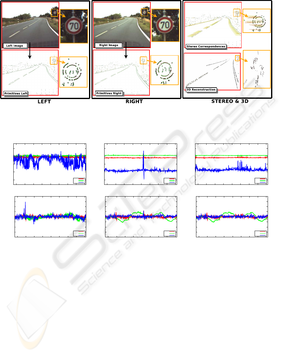
Figure 3: Extracted 2D and 3D primitives for a sample image pair. Note that, 2D primitives are used to reconstruct 3D

primitives.

Primitives SIFT Primitives and SIFT

−1500

−1000

−500

500

300 400 500 600 700 800 900 1000 1100

translation in mm

frame

s_06a_01#000: Primitives − Translation Parameters

−1500

−1000

−500

500

300 400 500 600 700 800 900 1000 1100

translation in mm

frame

s_06a_01#000: SIFT − Translation Parameters

−1500

−1000

−500

500

300 400 500 600 700 800 900 1000 1100

translation in mm

frame

s_06a_01#000: Combined − Translation Parameters

−0.02

−0.015

−0.01

−0.005

0.005

0.01

0.015

0.02

300 400 500 600 700 800 900 1000 1100

rotation in radians

frame

s_06a_01#000: Primitives − Rotation Parameters

−0.02

−0.015

−0.01

−0.005

0.005

0.01

0.015

0.02

300 400 500 600 700 800 900 1000 1100

rotation in radians

frame

s_06a_01#000: SIFT − Rotation Parameters

−0.02

−0.015

−0.01

−0.005

0.005

0.01

0.015

0.02

300 400 500 600 700 800 900 1000 1100

rotation in radians

frame

s_06a_01#000: Combined − Rotation Parameters

Figure 4: Motion estimation results for different feature sets over the entire stereo image sequence (frame 267-1116).

cases, only one of these predictions will be conﬁrmed

by the visual representation observed at instant t + δt.

This means that, over a few frames, stereo correspon-

dences can be disambiguated by tracking. We com-

bined the tracking information into one accumulated

likelihood measure that we use to discard unlikely hy-

potheses (Pugeault et al., 2008). On the other hand,

primitives that achieve a high enough likelihood are

ﬂagged as correct, and preserved even if they there-

after leave the ﬁeld of view or become occluded.

4.2 Spatial Disambiguation via NURBS

Parametrization

The second disambiguation scheme employed here

is using the collinear groups formed in both images.

Stereo matches that do not agree with the group struc-

ture of a primitive are discarded, leading to a reduc-

tion of ambiguity (Pugeault et al., 2006).

Moreover, it is advantageous to have an explicit

parameterization of collinear groups to allow for a

controlled and more condensed description of such

entities as well as for having a good control over pa-

rameters such as position, orientation and curvature

along these structures. NURBS (Non-uniform Ratio-

nal B-Splines) (Piegl and Tiller, 1995) has been cho-

sen as a suitable mathematical framework since it is

invariant under afﬁne as well as perspective trans-

formations, can be handled efﬁciently in terms of

memory and computational power and offer one com-

mon mathematical form for both standard analytical

shapes and free-form shapes. Note that, these proper-

ties hold true for 3D as well as 2D data.

NURBS parametrization is not used only for an-

ROAD INTERPRETATION FOR DRIVER ASSISTANCE BASED ON AN EARLY COGNITIVE VISION SYSTEM

499

-1500

-1000

-500

500

300 400 500 600 700 800 900 1000 1100

translation in mm

frame

s_06a_01#000: Combined Filtered - Translation Parameters

-0.02

-0.015

-0.01

-0.005

0.005

0.01

0.015

0.02

300 400 500 600 700 800 900 1000 1100

rotation in radians

frame

s_06a_01#000: Combined Filtered - Rotation Parameters

Figure 5: Motion estimation results after applying Bootstrap ﬁlter to results in Figure 4.

Figure 6: Position and orientation correction of 3D features by using NURBS. Green lines represent NURBS and black lines

represent groups of features.

alytical calculations that are necessary to create the

lane parametrization described in Section 6, but also

used for disambiguation in terms of position and ori-

entation correction of 3D features. The correction

procedure is illustrated in Figure 6. After ﬁtting

NURBS (represented as green lines) to groups of 3D

features (represented as black lines), position and ori-

entation of each feature is recalculated. The proce-

dure is shown on a good reconstruction (middle road

marker) as well as a bad one (left lane marker).

5 LARGE SCALE SEMANTIC

MAPS

One additional information provided by tracking is

that it allows us to identify new information that is not

tracked yet. All observed 3D-primitives that are not

matched with one pre-existing, tracked 3D-primitive

are added to the accumulated representation. This

allows for integrating visual information over larger

scales (Pugeault et al., 2008), in a manner similar to

SLAM applications. The difference being here that

the features densely describe the shape of the visual

world, rather than being mere clouds of landmarks.

This allows, over a scale of a few seconds for gen-

erating a richer representation of more global driv-

ing events, like road curvature, and the car’s trajec-

tory. The accumulated representation on the driving

sequence in Figure 2 is shown in Figure 7, from dif-

ferent perspectives and at different points of the road.

The ﬁrst (top-left) image shows the whole road seg-

ment (in perspective).

VISAPP 2009 - International Conference on Computer Vision Theory and Applications

500

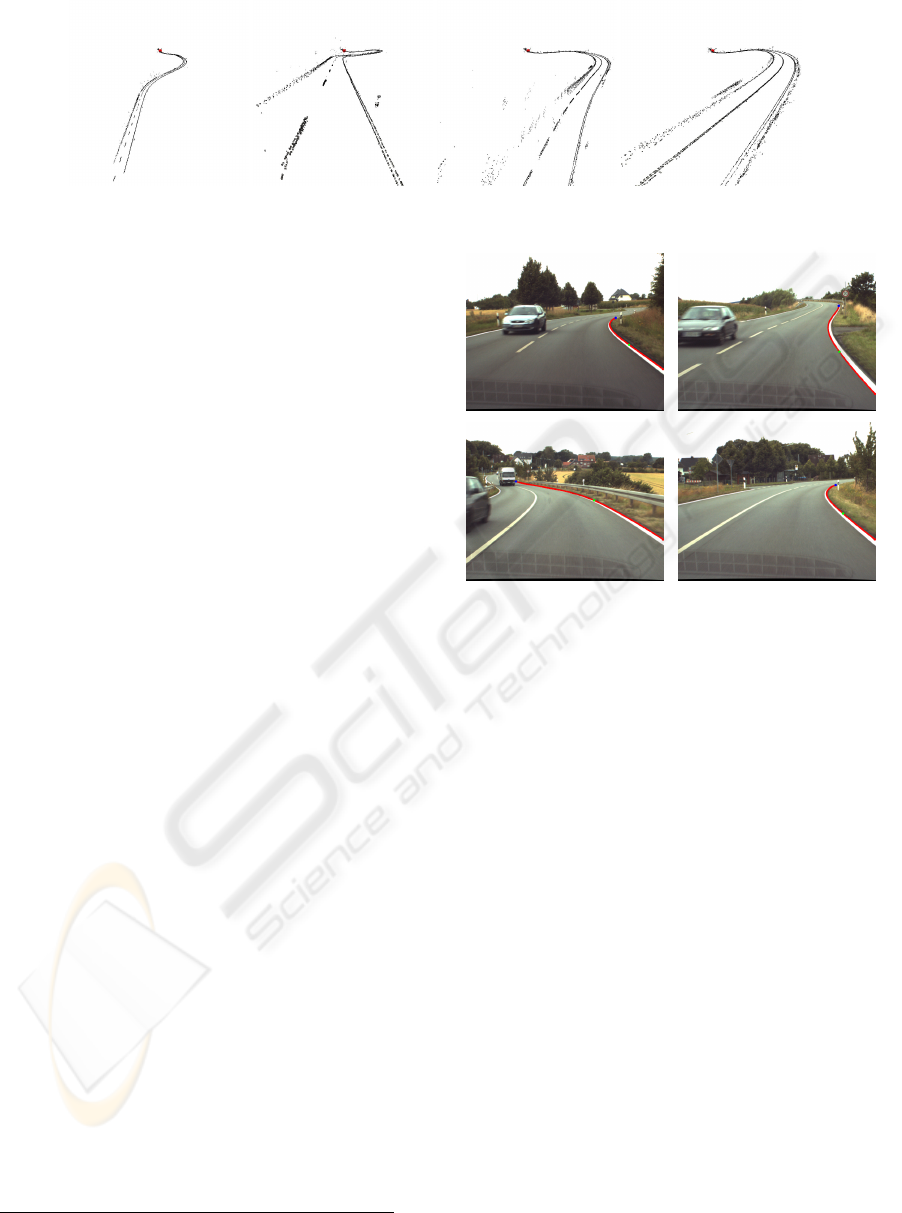
Figure 7: Large scale accumulation: four different viewpoints on the accumulated maps after 1000 frames ( 40s.).

6 BAYESIAN LANE FINDING

AND PARAMETRIZATION

In this section, a framework for ﬁnding road

lane markers based on Bayesian reasoning and

parametrization of the lanes in terms of feature vec-

tors are discussed. The visual representation dis-

cussed in Section 2 does not only provide local im-

age features but also provides relations between these

features (Bas¸eski et al., 2007) (e.g., proximity, cocol-

ority, distance). We want to ﬁnd the primitives con-

stituting the lane in a process combining the different

relations.

To merge the different cues/relations as well as to

deal with the uncertainties present in a vision system,

we make use of a Bayesian framework. The advan-

tage of Bayesian reasoning is that it allows us to:

• make explicit statements about the relevance of

properties/relations for a certain object,

• introduce learning in terms of prior and condi-

tional probabilities, and

• assess the relative importance of each type of re-

lation for the detection of a given object, using the

prior probabilities.

Let P(e

) be the prior probability of the occur-

rence of an event e

(e.g., the probability that a primi-

tive lies in the ground plane, or that two primitives are

coplanar, collinear or have a certain distance to each

other).Then, P(e

|Π ∈ O) is the conditional probabil-

ity of the visual event e

given an object O.

Our aim is to compute the likelihood of a primitive

Π being part of an object O given a number of visual

events relating to the primitive:

P(Π ∈ O |e

). (3)

According to Bayes formula, equation 3 can be

expanded to:

P(e

|Π ∈ O )P(Π ∈ O)

P(e

|Π ∈ O )P(Π ∈ O) + P(e

|Π /∈ O )P(Π /∈ O)

(4)

Figure 9: Extracted right lanes (shown in red) for some im-

ages in the reference sequence.

Using this framework for detecting lanes, we ﬁrst

need to compute prior probabilities. This is done by

hand selecting the 3D primitives being part of a lane

in a range of scenes and calculating the different rela-

tions and attributes for these selections. The resulting

probabilities will reveal which relations and attributes

are relevant for detecting this object.

Figure 8 shows the results of using the Bayesian

framework with the relevant relations for detecting

lane markers in an outdoor scene.

After ﬁnding the 3D features that potentially be-

long to the road by using Bayesian reasoning, the

right lane of the road is extracted by using small

heuristics in 2D. Since the lane starts as two sepa-

rate stripes and becomes a single line further from the

camera, we eliminate the short groups that are neigh-

bor to a long group if the color distribution between

the two groups is uniform. After eliminating the short

groups, we select the group closest to the bottom-right

corner of the image as the right lane. Note that, al-

though the potential street lanes were found in 3D via

Bayesian reasoning, the hierarchy in the representa-

tion allows us to do reasoning in 2D for the last step

by using the link between 3D and 2D groups. In Fig-

ure 9, some results that show the right lane of the road

are presented. Once the right lane of the road is de-

ROAD INTERPRETATION FOR DRIVER ASSISTANCE BASED ON AN EARLY COGNITIVE VISION SYSTEM

501

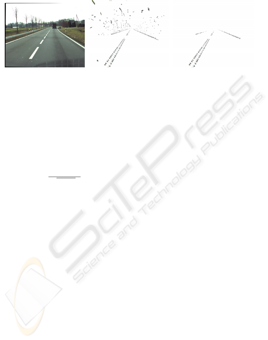
(a) Original outdoor image (b) Extracted primitives (c) Selected primitives

Figure 8: Extracting the lane in an outdoor scenario

tected, it is necessary to create a parametrization of

the lane so that it can be used for driver assistance.

The idea is to represent certain locations of the lane

as a feature vector, depending on the dimension of

the data. In 2D, the feature vector is v

= [x

,κ

]

where x

is the x coordinate corresponding to a ﬁxed

y coordinate y

on the lane and κ

, s

are the curvature

and slope at point (x

) respectively. Note that, for

a curve given parametrically as c(t) = (x(t), y(t)), the

curvature is deﬁned as:

κ =

− y

(

+ y

)

(5)

In 3D, the feature vector is V

= [X

, j

] where

) is the x and y coordinates corresponding to

a ﬁxed Z coordinate Z

on the lane and [i

, j

] is

the tangent vector at point (X

). Note that, ﬁt-

ting NURBS to the right lane plays an important role

in these calculations since it allows applying similar

procedures for both 2D and 3D data. Also, analytical

calculations like derivation is more stable and easy to

compute when NURBS is used.

In Figure 10(d-f), the 2D lane parameter extrac-

tion results are presented for the reference sequence

collected from the road shown in Figure 2. For each

image in the sequence, a 2D feature vector has been

found from the right lane for y coordinate equals to

500 pixels. The road has two sharp right turns and

one less sharp left turn with the order right, left, right.

The plots regarding the slope and x coordinate show

all three turns as shown in Figure 10 (d) and (e). On

the other hand, the plot for curvature (Figure 10 (f))

can show only two sharp right turns and gives slight

indication of left turn. Position and tangent vector de-

scribe the structure of the road in 3D as well, as shown

in Figure 10 (a) and (c).

7 INDEPENDENTLY MOVING

OBJECTS

One important source of information in a driving con-

text lies with the other vehicles (and more generally

all other moving objects), their detection, tracking and

identiﬁcation. In this work, Independently Moving

Objects (IMOs) are detected by subtracting the optic

ﬂow introduced by the car’s self-motion from the ob-

served optical ﬂow as described in (Pauwels, 2008).

This provides a list of IMOs, with appropriate bound-

ing boxes (BB). We use this information to segment

the image in areas (background and IMOs) where vi-

sual information is extracted and accumulated sepa-

rately (as in Section 4.1).

Figure 11 illustrates the IMO handling module of

the system. In (a) the detected IMOs are identiﬁed

by bounding boxes and an unique ID; (b) the left im-

age patch contained in the IMO’s BB is extracted and

magniﬁed to increase resolution; (c) the right BB’s

location is estimated using the mean disparity of the

primitives in the left BB, and the corresponding patch

in the right image is also extracted and magniﬁed; (d)

new primitives are extracted on the magniﬁed images

and matched across both patches. The stereo matches

are used for reconstructing 3D-primitives, as before,

and accumulated over time.

Figure 12 shows the segmentation of the IMOs.

On the left, the ﬁgure shows a detail of the accumu-

lated road. The IMO has been segmented out. On

the right the accumulated representation of the IMO

is also displayed in the same coordinate system. Fig-

ure 13 shows the accumulated background and one

of the IMOs, with the associated trajectories (rep-

resented as the red and green string of arrows); (a)

shows only the accumulated background and the ego-

motion; (b) and (c) also show the accumulated IMO

and its trajectory; (d) shows the IMO’s estimated tra-

jectory, from above. The car’s egomotion averages

to 65 km/h on this sequence, whereas the IMO’s mo-

VISAPP 2009 - International Conference on Computer Vision Theory and Applications

502

(b) (c)

(d)

(f)(e)

frame

position

(a)

tangent

frame

tangent

frame

position

frame

curvature

−0.02

−0.015

−0.01

−0.005

0.005

0.01

0.015

0.02

300 400 500 600 700 800 900 1000 1100

rotation in radians

frame

−5000

5000

10000

15000

20000

25000

30000

200 300 400 500 600 700 800 900 1000 1100 1200

POSITION_y

POSITION_x

POSITION_z

0.1

0.2

0.3

0.4

0.5

0.6

0.7

0.8

0.9

200 300 400 500 600 700 800 900 1000 1100 1200

TANGENT_i

TANGENT_j

TANGENT_k

200 300 400 500 600 700 800 900 1000 1100 1200

200

300

400

500

600

700

800

900

1000

1100

200 300 400 500 600 700 800 900 1000 1100 1200

−0.015

−0.01

−0.005

0.005

0.01

0.015

0.02

200 300 400 500 600 700 800 900 1000 1100 1200

Figure 10: Motion of the car from different sources (2D-3D lane parameters and ego motion estimation). (a)-(c) (x,y,z)

coordinates and components of the tangent vector of the 3D lane for z = 25meters on the whole reference sequence. (b) Ego

motion estimation for rotation by using combination of SIFT and primitives. (d-f) 2D lane parameters for y = 500pixels on

the whole reference sequence. (d) slope (e) x coordinate (f) curvature.

Figure 11: IMOs processing. (a) IMO list and BBs (b) left image segment, (c) right image segment, (d) extracted primitives

and stereo correspondences.

ROAD INTERPRETATION FOR DRIVER ASSISTANCE BASED ON AN EARLY COGNITIVE VISION SYSTEM

503

Figure 12: Segmentation and reconstruction of an IMO: left shows the accumulated map of the road, where IMOs are seg-

mented out; right shows the accumulated representation of the IMO, on the same coordinate system.

Figure 13: One IMO in a semantic map and its trajectory. (a) shows only the accumulated background and the car’s egomotion;

(b) and (c) show in addition the accumulated IMO and its trajectory, under different viewpoints; and (d) shows the IMO’s

trajectory viewed from above.

tion averages at 80 km/h. In those results one see

that the IMOs can be segmented and tracked. The use

of dense method for detection and tracking provides

robustness, and the use of symbolic features for accu-

mulation provides consistency to the system.

8 CONCLUSIONS

We have discussed four algorithms as sub-parts of a

road interpretation, based on visually extracted data,

provided by an early cognitive vision system. After

increasing the reliability of 2D and 3D information

by using temporal and spatial disambiguation mecha-

nisms, lane markers of the road are detected and the

ego-motion of the car is estimated. While having the

ego-motion in hand, large scale maps of the road and

independently moving objects on the road are created.

The potential of the presented algorithms has been

demonstrated on a stereo image sequence, collected

from a structured road. We have shown that the resul-

tant large scale map, as well as the estimated motion

and the detected lane parameters are consistent with

the satellite image. Note that, all sub-tasks use only

visually extracted information and all parts of this in-

formation are provided by the same representation.

ACKNOWLEDGEMENTS

This work has been supported by the European Com-

mission - FP6 Project DRIVSCO (IST-016276-2) and

the national Danish project NISA.

REFERENCES

Bas¸eski, E., Pugeault, N., Kalkan, S., Kraft, D., W

org

otter,

F., and Kr

uger, N. (2007). A Scene Representation

Based on Multi-Modal 2D and 3D Features. ICCV

2007 Workshop on 3D Representation for Recognition

3dRR-07.

Bertozzi, M. and Broggi, A. (1998). GOLD: A Parallel

Real-Time Stereo Vision System for Generic Obstacle

and Lane Detection. Image Processing, IEEE Trans-

actions on, 7(1):62–81.

Bertozzi, M., Broggi, A., and Fascioli, A. (2000). Vision-

based Intelligent Vehicles: State of the Art and

VISAPP 2009 - International Conference on Computer Vision Theory and Applications

504

Perspectives. Robotics and Autonomous Systems,

32(1):1–16.

Faugeras, O. (1993). Three-Dimensional Computer Vision:

A Geometric Viewpoint. MIT Press.

Fischler, R. and Bolles, M. (1981). Random Sample Con-

sensus: A Paradigm for Model Fitting with Applica-

tions to Image Analysis and Automated Cartography.

Communications of the ACM, 24(6):619–638.

Gordon, N., Salmond, D., and Smith, A. (1993). Novel

Approach to nonlinear/non–Gaussian Bayesian State

Estimation. In IEE Proceedings-F, volume 140, pages

107–113.

Hermann, S. and Klette, R. (2008). A Study on Parameteri-

zation and Preprocessing for Semi-Global Matching.

Technical Report Number 221, Computer-Science

Department of The University of Auckland, CITR.

Jensen, L. B. W., Kjær-Nielsen, A., Alonso, J. D., Ros, E.,

and Kr

uger, N. (2008). A Hybrid FPGA/Coarse Par-

allel Processing Architecture for Multi-modal Visual

Feature Descriptors. ReConFig’08.

Klette, R. (2008). Stereo-Vision-Support for Intelligent Ve-

hicles - The Need for Quantiﬁed Evidence. Technical

Report Number 226, Computer-Science Department

of The University of Auckland, CITR.

uger, N., Lappe, M., and W

org

otter, F. (2004). Bi-

ologically Motivated Multi-modal Processing of Vi-

sual Primitives. The Interdisciplinary Journal of Ar-

tiﬁcial Intelligence and the Simulation of Behaviour,

1(5):417–428.

Leibe, B., Cornelis, N., Cornelis, K., and Van Gool, L.

(2007). Dynamic 3D Scene Analysis from a Moving

Vehicle. Computer Vision and Pattern Recognition,

2007. CVPR ’07. IEEE Conference on, pages 1–8.

Lemaire, T., Berger, C., Jung, I.-K., and Lacroix, S.

(2007). Vision–Based SLAM: Stereo and Monocu-

lar Approaches. International Journal of Computer

Vision, 74(3):343–364.

Lowe, D. (2004). Distinctive Image Features from Scale-

Invariant Keypoints. International Journal of Com-

puter Vision, 2(60):91–110.

McCall, J. and Trivedi, M. (2004). An Integrated, Robust

Approach to Lane Marking Detection and Lane Track-

ing. pages 533–537.

Pauwels, K. (2008). Computational Modeling of Visual At-

tention:Neuronal Response Modulation in the Thala-

mocortical Complex and Saliency-based Detection of

Independent Motion. PhD thesis, K.U.Leuven.

Pauwels, K. and Van Hulle, M. M. (2008). Optic Flow from

Unstable Sequences through Local Velocity Con-

stancy Maximization. Image and Vision Computing,

page in press.

Piegl, L. and Tiller, W. (1995). The NURBS Book. Springer-

Verlag, London, UK.

Pugeault, N., W

org

otter, F., and Kr

uger, N. (2006). Multi-

modal Scene Reconstruction Using Perceptual Group-

ing Constraints. In Proc. IEEE Workshop on Percep-

tual Organization in Computer Vision (in conjunction

with CVPR’06).

Pugeault, N., W

org

otter, F., and Kr

uger, N. (2008). Accu-

mulated Visual Representation for Cognitive Vision.

In Proceedings of the British Machine Vision Confer-

ence (BMVC).

Rosenhahn, B., Kr

uger, N., Rabsch, T., and Sommer, G.

(2001). Automatic tracking with a novel pose estima-

tion algorithm. Robot Vision 2001.

Wang, Y., Teoh, E., and Shen, D. (2004). Lane Detection

and Tracking Using B-Snake. 22(4):269–280.

ROAD INTERPRETATION FOR DRIVER ASSISTANCE BASED ON AN EARLY COGNITIVE VISION SYSTEM

505