From Reactive to Deliberative Multi-agent Planning

Ammar Mohammed and Ulrich Furbach

Universit¨at Koblenz-Landau, Computer Science Department, Koblenz, Germany

Abstract. Various researches approached hybrid automata to formally model

and coordinate reactive multi-agent systems’ plans situated in a dynamic environ-

ment, where the time is critical. However in most of cases, reactivity in dynamic

environments is not satisfactory. It is favorable that agents plan their behaviors

according to some preference function. Most of current veriﬁcation tools of hy-

brid automata are inadequate to model such agents’ plans. Therefore, this paper

extends hybrid automata’s decisions making by means of utility functions on tran-

sitions. A scenario taken from supply chain management is demonstrated to show

the paper’s approach. Analysis of agents’ plans are investigated using a constraint

logic program implementation prototype.

1 Motivation

Multi-agent planning [2] is a demanded task especially in a safety critical environ-

ment, where unexpected events typically arise. One key characteristics of multi-agent

planning is the nature of the environment in which the agents are involved. In realistic

problems, the environment tends to be dynamic and the behaviors of the agents change

continuously in their environment. Planning in this dynamical environment is called

continual planning [3]. Agents should engage in continual planning, if agents’ objec-

tives can evolve over time, where the purpose of the planning is to set a target that can

be achieved based on a given set of constraints at a given time. Therefore, it is becoming

increasingly important for the agents to react to the unexpected events, appeared during

the planning, in real time in order to avoid the risk that may occur during the planning.

However, agents should not only react to change those events that threaten the execu-

tion of the plan, but also coordinate for opportunities to improve the plan by taking into

account the expected future development in order to decide the most favorable course

of actions based on utility functions. Hence, there is a need to a formal way to model

and analysis the multi-agent planning in dynamical environments that combined both

aspects in a single framework.

Hybrid automata [8], on the other hand, can be used to model multi-agent systems

plans that are deﬁned through their capability to continuously react in dynamic envi-

ronments, while respecting some time constraints. Therefore, there are researches, for

example [13,4, 5], which have proposed hybrid automata to formally model reactive

multi-agent systems [6]. There are authors, for example [10], who have approached a

simple form of hybrid automata that are called timed automata [1] to model reactive

agents. However, in reactive agents, decisions making depend entirely on the occur-

rence of events, where the agents base their next states on their current sensory events.

Mohammed A. and Furbach U. (2009).

From Reactive to Deliberative Multi-agent Planning.

In Proceedings of the 7th International Workshop on Modelling, Simulation, Veriﬁcation and Validation of Enterprise Information Systems, pages 67-75

DOI: 10.5220/0002192700670075

 SciTePress

In contrast to reactive agents, deliberative/rational agents take into account the expected

future development in order to decide the most favorable course of actions based on

utility functions. Decisions making of deliberative agents are inadequately expressive

to hybrid automata. To our knowledge, current hybrid automata tools, like [9,7,12], do

not offer help for efﬁciently modeling these types of situations. Therefore, it seems to

be useful to extend hybrid automata in a way that they allow the combination of reactive

and deliberative decisions making. This combination can avoid catastrophic failure, and

provide good quality of decisions in time constrained dynamical environments. Conse-

quently, the formal veriﬁcation of hybrid automata, by means of reachability analysis,

can be used as planning-problem solver, where a plan can be achieved, iff the ﬁnal plan

is reachable.

To this end, this paper contributes to enhance the decision making of the hybrid

automata by coordinating their plans in dynamic environments to improve their future

outcomes . This can be accomplished by allowing discrete transitions occurring on the

basis not only of reactive decisions, but also of preference functions. We use our con-

straint logic program (CLP) implementation prototype [14]

to demonstrate the contri-

bution. The expressiveness of CLP facilitate this extension. Additionally, an example

taken from supply chain management in continuous dynamic environment is depicted.

As far as we know, this is the ﬁrst attempt to use hybrid automata to plan multi-agent

systems with decisions making rely on a performance measurement.

In the sequel, we ﬁrst introduce a case study that will be used throughout the paper

to illustrate our approachin Sec. 2. Then formaldeﬁnitions of extended hybridautomata

are discussed in Sec. 3. Sec. 4 brieﬂy shows the basic structure of our CLP implemen-

tation model, before showing how to specify and verify the planning requirements in

Sec. 5. Eventually, we end up with the conclusion in Sec. 6

2 Case Study

To this end, this section demonstrates a logistic scenario in a continuous dynamic envi-

ronment and shows how to specify it as hybrid automata. In this scenario, a customer

has a shipment of decayable freight items that has to be transported to some destina-

tion point. Therefore, s/he contacts a transportation service provider for this mission.

The transportation service provider, in turn, assigns a transportation truck to convey the

shipment. Assuming that the customer signs a contract with the service provider so that

the freight items have to delivered with certain threshold

of items’ quality (e.g. at

most 20% putrefaction of the freight items). Otherwise, the provider has to recompense

the customer with a convenient deal. Therefore, for quality assurance and provider’s

proﬁtable service constraints, the quality of freight items has to be monitored in the

truck during the transportation. In case of an exception (e.g. cooling temperature breaks

down), the truck has to ﬁnd a suitable plan to deal with this exception, but taking into

account to utilize its transportation provider business.

Extended version with benchmarks results will appear in proceeding of the 7th International

Workshop on Programming Multi-Agent Systems (ProMAS 2009) at the eighth International

Joint conference on Autonomous Agents & Multi-Agent Systems (AAMAS 2009)

unsafe

stable

decay

System

init

Monitor

Truck

propose

init

transport estimate

w help

continuearrived

Provider

w propose to target w rescue

target

Disturbance

init

disturb

no disturb

init

error

D = 0

violate

ﬁnish

D ≤

Y := 0

Y = 0

D := 0

Y = 1

erroraccept

ﬁnish

Z = 0

Z = 1

Z := 0

cfp

help

ﬁnish

X := 0

X = 0

X = 50

X = 0

X ≤ d

X = 50

X ≤ d

cfp

X = d

X = 0

ﬁnish

error

rescueﬁnish

ﬁnish

help

:= f(d

, ˙x)

time

< Ex

ﬁnish

Z ≤ 2

Z ≥ 2

rescue

tosafeC

time

≥ Ex

rescued

ﬁnish

tosafe

error

tosafe

D = 1.2D

D := 1.2

D = 0

D ≥

Y ≥ t

Y ≤ t

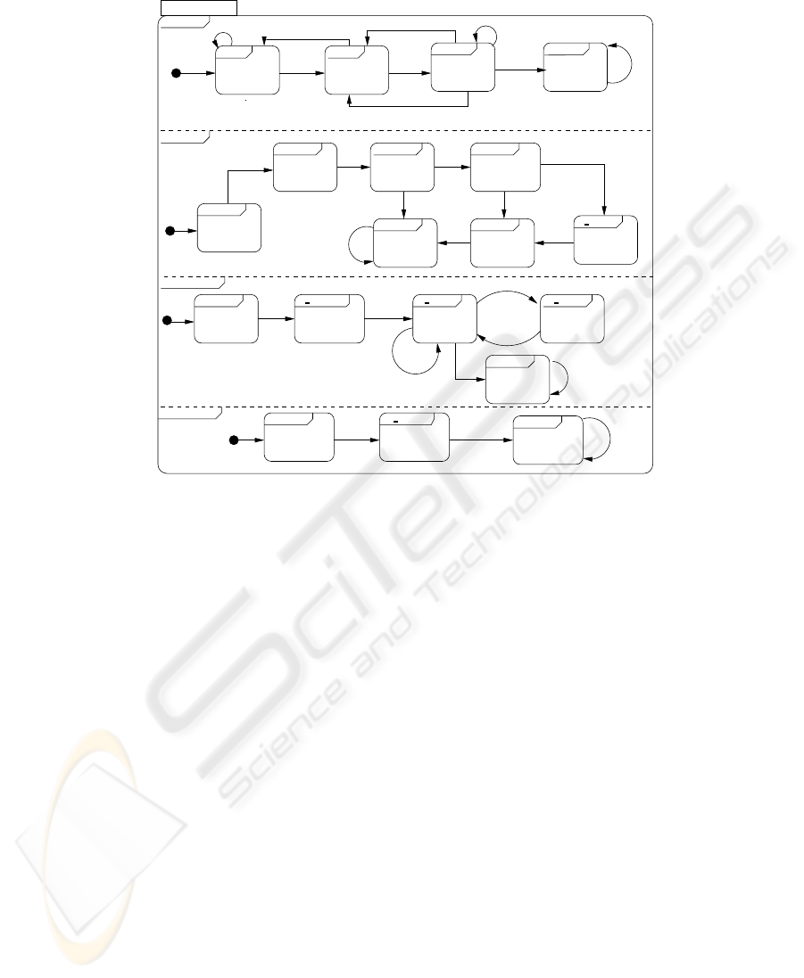
Fig.1. Speciﬁcation of a logistic scenario as hybrid automata.

In Fig. 1, the speciﬁcation of the previous multi-agent scenario is depicted as hybrid

automata - Due to the space limitation, the description of each automaton will not be

elaborated in details-. The multi-agent scenario constitutes four agents, Monitor, Truck,

Provider, and Disturbance. The agent Monitor, plugged into the truck, observes the oc-

currence of exceptional errors, as well as the putrefaction of the items. The items are

putreﬁed according to the exponential decay function, given as

D = 1.2 ∗ D. When an

exceptional error occurs during the transportation, which is stimulated by the Distur-

bance agent after some time t

, the Monitor agent alarms the Truck with the occurrence

of this error. In turn, the Truck has to make an appropriate decision before the decayed

items reach a certain threshold

. The decision is estimated, using the variable Ex

according to the remaining distance to the destination point. Here, Ex

is calculated

based on the dynamic of distance of the truck to the target. If the expected delivery

time is beyond a given critical time C

time

, then the Truck requests help from the trans-

portation service provider, who sends a rescue truck within two hours. However, if the

truck estimation is below the critical time C

time

, then it should continuously transport

the shipment according to the current conditions. At the end of transportation, both the

customer and the provider check the result of the previous plan.

The objective of the previous scenario is to check that the agents, particularly the

truck, will choose the right plan during the course of execution that utilize the proﬁt of

its provider company.

3 Hybrid Automata

This section shows the basics extension to the syntax and semantics of hybrid automata.

A hybrid automaton is represented graphically as a state transition diagram dialect like

statecharts, augmented with mathematical formalisms on both transitions and locations.

Formally, a hybrid automaton/agent is deﬁned as follows.

Deﬁnition 1 (components). A hybrid automaton is a tuple H =

(Var, Q, Inv, Flow, Init, E, Jump, Event,

, Assgn) where:

– Var = R∪ A is a set of variables, where R ⊆ ℜ

is a ﬁnite set of n real-valued vari-

ables that model the continuous dynamics, whereas A is a set of auxiliary variables

that are used as a performance measure to make a decision. For example, the Truck

automaton has X ∈ R and Ex

∈ A.

– Q is a ﬁnite set of control locations. For example, the Disturbance automaton Fig. 1

has the locations init, no disturb,and disturb.

– Inv(q) is the invariant predicate, which assigns a constraint to the dynamic vari-

ables R ⊆ Var for each control location q ∈ Q. The control of a hybrid automaton

remains at a location q ∈ Q, as long as Inv(q) holds. For instance, the location

decay in the Monitor automaton has the invariant D ≤

. Omitting the invariant at

some location indicates that the location is always achievable.

– Flow(q) is the ﬂow predicate on the dynamic variables R ⊆ Var for each control

location q ∈ Q, which deﬁnes how the variables in R evolve over the time at location

q. It constrains the time derivative of the continuous part of the variablesat location

q. The ﬂow of a variable X is denotedas

X. For example,

X = 50 describes the speed

of the automaton Truck at the location transport.

– Init is the initial condition that assigns an initial values to the variables R ∈ Var to

each control location q ∈ Q. For example, X = 0 is the initial condition of the Truck

automaton.

– E ⊆ Q× Q is the discrete transition relation over the control locations. Each edge

e = (q

, q

) ∈ E is augmented by the following annotations:

Jump: jump condition (guard), which is a constraint over Var that must hold upon

ﬁring a transition e.

Event: synchronization label, used to synchronize concurrent automata. The syn-

chronization labels deﬁne how the automata are coordinated in terms of the

parallel composition.

Utility cost, which captures the preference of an agent over e. Formally, this is

done by introducing the function

: E → ℜ. For example, at the location es-

timate, the Truck has preferences to go to either location w help or continue,

with utilities

and

respectively. The utility cost is omitted if there is no

preference on the edge e.

– Assgn is the updating function Assgn : R∪ A → ℜ, which resets the variables before

the control of a hybrid automaton goes from location q

to location q

. It is denoted

as v := Assgn(v). Here, we graphically distinguish between two types of updating

depending on types of variables v ∈ Var. Case v ∈ R (i.e. updating continuous vari-

ables), then the update is annotated graphically on the transitions e = (q

, q

). For

example, D := 1.2 is the updating of the continuous variable D between location

stable and decay in the automaton Monitor. Updating the variables on transitions

are omitted, if the value of the variables at end of location q

are the same at the

beginning of location q

. On the other hand, case v ∈ A (i.e. updating auxiliary

variables), then the update is annotated inside location q

. The reason behind this

is that these variables will be used afterward as decisions making on transitions.

For example, in the location estimate of the Truck automaton, EX

:= f (d

, ˙x) is

updating the auxiliary variable EX

to the estimated remaining time to deliver the

shipment to the target based on the current remaining distance to the target.

Semantically, both types of updates are the same. This is because both of them will

be eventually executed before the control goes immediately to location q

Informally speaking, the semantics of a hybrid automaton is deﬁned in terms of a la-

beled transition system between states, where a state consists of the current location of

the automaton and the current valuation of the real variables. To formalize the seman-

tics of the hybrid automaton, we ﬁrst need to deﬁne the concept of a hybrid automaton’s

state.

Deﬁnition 2 (State). At any instant of time, a state of a hybrid automaton is given by

= hq

, v

,ti, where q

∈ Q is a control location, v

is the valuationof the real variables,

and t is the current time. A state

= hq

, v

,ti is admissible if Inv(q

)[v

] holds.

A state transition system of a hybrid automaton H starts with the initial state

, v

, 0i, where the q

and v

are the initial location and valuations of the variables

respectively. For example, the initial state of the Truck (Fig. 1) can be speciﬁed as

hinit, 0, 0i.

Since we need to extend the agent decisions by means utilities, here we deﬁne the

term preference.

Deﬁnition 3 (Preference).Let q ∈ Q is a control location, whose preferences with con-

trol locations {q

, q

, .., q

} with respective utilities {

, ..,

}. We call q

is the best

preference location to q if

= Max{

, ..,

}

Intuitively, an execution of a hybrid automaton corresponds to a sequence of transitions

from one state to another. In fact, a hybrid automatonevolvesdepending on two kinds of

transitions: continuous transitions, capturing the continuous evolution of states, and dis-

crete transitions, capturing the decision making to change into another location. More

formally, we can deﬁne hybrid automaton operational semantics as follows.

Deﬁnition 4 (Operational Semantic). A transition rule between two admissible states

= hq

, v

i and

= hq

, v

i is deﬁned as follows:

discretely: iff t

= t

and Jump(v

) holds, then variables are reset at location q

such

that, Inv(q

)[v

] holds. Additionally, q

is the best preference of q

. In this case an

event a ∈ Event may be ﬁred.

continuously(time delay): iff q

= q

, and (t

− t

> 0) is the duration of time passed

at location q

, during which the invariant predicate Inv(q1) continuously holds,

, v

are the variable valuations according to the ﬂow predicate Flow(q1).

In principle, an execution of a hybrid automaton corresponds to a sequence of transi-

tions from one state to another, therefore we deﬁne the valid run as follows.

Deﬁnition 5 (Run). A run of hybrid automaton

∑

.., is a ﬁnite or inﬁnite

sequence of admissible states, where

is the initial state.

In a run

∑

, the transition from a state

to a state

i+1

is related by either a discrete or

a continuous transition, according to Def. 4.

It should be noted that the continuous change in the run may generate an inﬁnite

number of reachable states. It follows that state-space exploration techniques require a

symbolic representation system for the sets of states that have to be manipulated (this

is implemented efﬁciently using our CLP model [14] by means of mathematical ﬁnite

interval). We call the symbolic interval a region. Consequently, the set of all reachable

states at location q ∈ Q can be represented as hq,V, Timei, where V and Time repre-

sent the reachable region and time at location q respectively. Now, the run of hybrid

automata can be re-stated as a form of reachable regions, where the change from one

region to another one is ﬁred using a discrete step.

The operational semantics is the basis for veriﬁcation of hybrid automata. In partic-

ular, model checking of a hybrid automaton is deﬁned in terms of reachability analysis

of the hybrid automaton.

Deﬁnition 6 (Reachability). A state

is reachable from a state

, if there is a se-

quence of admissible states starting from

and ending in

. A state

is called

reachable if it can be reached from the initial state

To model multi-agents system, one needs to coordinate the behaviors of the agents. For

this reason, hybrid automata can beextendedby parallel composition. Basically, parallel

composition of hybrid automata can be used for specifying larger systems (multi-agent

systems), where a hybrid automaton is given for each part of the system, and communi-

cation between the different parts may occur via shared variables and synchronization

labels. Technically, the parallel composition of hybrid automatais obtainedfrom the dif-

ferent parts using a product construction of the participating automata. The transitions

from the different automata are interleaved, unless they share the same synchronization

label. In this case, they are synchronized during the execution.As a result of the parallel

composition, an automaton is created, which captures the behavior of the entire system.

4 CLP Model

This section shows brieﬂy how to encode the hybrid automata described in the previous

section using our CLP model [14]. The key advantage of our implementation model in

contrast to the other hybrid automata veriﬁcation tools is that we do not need to con-

struct the composition of hybrid automata prior to veriﬁcation phase. Instead, we con-

struct the behaviors dynamically during the computation. This relieves the state space

problem that may occur when modeling multi-agent systems. The prototype was built

using ECLiPSe Prolog [11]. Due to the space limitation, we will omit some details, but

we will show the basic outline of the CLP model.

An automaton is deﬁned by a predicate ranging over the respective locations of the

automaton, real-valued variables, and the time:

automaton(Location,Vars,Vars0,T0,Time):-

c(Inv),c(Vars,Vars0,T0,Time).

Here, automaton is the name of the automaton itself, and Location represents is the

current location of the automaton. Vars is a list of real variables participating in the

automata, whereas Vars0 is a list of the correspondent initial values. c(Invs) is the

constraint that represents the invariant of the location, and the constraint predicate

c(Vars,Vars0, T0, Time) represents the continuous ﬂows of the variable Vars wrt. time

{T0, Time} , where T0 is the initial time at the start of the continuous ﬂow. The opera-

tional semantics are encode into CLP

evolve

predicate as follows.

evolve(Automaton,(L1,Var1),(L2,Var2),T0,Time,Event) :-

continuous(Automaton,(L1,Var1),(L1,Var2),T0,Time,Event);

discrete(Automaton,(L1,Var1),(L2,Var2),T0,Time,Event).

the

evolve

alternates between

continuous

and

discrete

based on the constraints that

appear during the run, as well as the Event that may occur.

Now, after the automata have been speciﬁed, a driver program is needed to coor-

dinate and execute the behaviors of the automata. For this reason, driver predicate is

implemented to do these missions. The last argument of the driver represents symboli-

cally the list of reachable regions.

driver((L1,Var01),(L2,Var02),...,(Ln,Var0n),T0,

[(L1,L2,..,Ln,Var1,Var2,..,Varn,Time,Event)|NextRegion]) :-

automaton1(L1,Var1,Var01,T0,Time1),

automaton2(L2,Var2,Var02,T0,Time2),

... ,

automatonn(Ln,Varn,Var0n,T0,Timen),

Time1 $=Time2, Time1 $=Time3, ..., Time1 $=Timen,

evolve(automaton1,(L1,Var01),(NextL1,Nvar01),T0,Time1,Event),

evolve(automaton2,(L2,Var02),(NextL2,Nvar02),T0,Time1,Event),

... ,

evolve(automatonn,(Ln,Var0n),(NextLn,Nvar0n),T0,Time1,Event),

driver((NextL1,Nvar01),(NextL2,Nvar02),...,(NextLn,Nvar0n),Time1,NextRegion).

To run the program, the driver has to be invoked with a query starting from the initial

states of the hybrid automata. An example, showing how to query the driver on logistic

multi-agent scenario, takes the form:

driver((init1,0),(init2,0),(init3,0),(init4,0),0,Reached).

5 Planning as Reachability Analysis

Now we have an executable constraint based speciﬁcation, which can be used to ver-

ify several properties of our multi-agent team by means of a reachability analysis. Let

Reached represents the set of reached regions, then in terms of CLP, the reachability

analysis can be generally speciﬁed by checking whether

Reached

holds, where

is the constraint predicate that describes a property of interest.

In the context of planning, the reachability question is equivalent to a plan existence.

For example, one can check that there is no bad plan, where the shipment is arrived to

its destination unsafely (i.e. the ratio of decayed items is below 20%). This can be in-

vestigated by showing that the location unsafe in the Monitor agent will not be reached.

Using the CLP computational model and with the help of the standard Prolog predicate

member/2, gives us the answer no as expected, after executing the following query:

?- drive((init1,0),(init2,0),(init3,0),(init4,0),0,Reached),

member((Monitor,_truck,_cargo,_disturbance,D,_x,_z,_y,Time,Event),

Reached),

Monitor = unsafe .

We are interested not only to ﬁnd a plan, but also to ﬁnd the plan that utilizes certain

tasks in case of happening an exceptional error. In the supply chain example, one can

check that the truck will choose the best plan that utilizes its company business and in

the same time fulﬁll the customer demands. This can be accomplished by investigating

the reachability of the shipment to its destination point with a certain precentage of

putrefaction D. For this purpose, the following query should be invoked.

?- drive((init1,0),(init2,0),(init3,0),(init4,0),0,Reached),

member((_monitor,Truck,_cargo,_disturbance,D,X,Z,Y,Time,Event),

Reached),

Truck = arrived.

However, there are several constraints, which inﬂuence the outcome of this query, such

as the time of the unexpected error generated by the Disturbance agent and the remain-

ing distance to the destination during the transportation. For example, setting the distur-

bance time t

= 8 in the supply chain model, the previous query gives the D ≃ 1.626%

upon the truck’s arrival to the destination, whereas setting t

= 24, the query gives

D ≃ 5.542%. In both cases, the customer’s demand is not violated according to the deal

with the provider. However, the contrast between the two values of D results from the

truck’s decision based on the constraintsappeared in the environment. In the ﬁrst case of

, the truck requested a rescue from the provider. However in the second case, the truck

remains transporting the shipment without requesting a help. The previous analysis can

be checked using the following query:

?- drive((init1,0),(init2,0),(init3,0),(init4,0),0,Reached),

member((_monitor,_truck,_cargo,_disturbance,D,X,Z,Y,Time,Event),

Reached),

Event = rescue.

This query checks the reachability of a state where an event rescue is reached. In other

words, the query means does the truck need a rescue?. In the ﬁrst case of t

, the query

returns with answer Yes, but it returns No in the second case.

6 Conclusions

Planning in dynamic environments is an essential task. Especially, when an exception

occurs during the planning. For this purpose, this paper showed how to extend the de-

cision making of hybrid automata on the base of performance functions for the unex-

pected events that occur during planning in dynamic environments. The extension was

illustrated by a scenario taken from supply chain management. Our CLP implementa-

tion model, helped us to achieve this extension ﬂexibly.

As a future work, we intend to experiment and relate our work to the other works of

multi-agent planning in dynamic environments, where the time is critical.

References

1. R. Alur and D. Dill. A Theory of Timed Automata. Theoretical Computer Science,

126(2):183–235, 1994.

2. M. de Weerdt, A. ter Mors, and C. Witteveen. Multi-agent planning: An introduction to

planning and coordination. Handouts of the European Agent Summer School, pages 1–32,

2005.

3. M. desJardins, E. Durfee, C. Ortiz Jr, and M. Wolverton. Survey of research in distributed,

continual planning. AI MAG, 20(4):13–22, 1999.

4. M. Egerstedt. Behavior Based Robotics Using Hybrid Automata. Lecture Notes in Computer

Science, pages 103–116, 2000.

5. A. El Fallah-Seghrouchni, I. Degirmenciyan-Cartault, and F. Marc. Framework for Multi-

agent Planning Based on Hybrid Automata. Lecture Notes in Computer Science, pages 226–

235, 2003.

6. J. Ferber and A. Drogoul. Using reactive multi-agent systems in simulation and problem

solving. Kluwer Computer And Information Science Series, pages 53–80, 1992.

7. G. Frehse. PHAVer: Algorithmic veriﬁcation of hybrid systems past HyTech. In M. Morari

and L. Thiele, editors, Hybrid Systems: Computation and Control, 8th International Work-

shop, Proceedings, LNCS 3414, pages 258–273. Springer, 2005.

8. T. Henzinger. The theory of hybrid automata. In Proceedings of the 11th Annual Symposium

on Logic in Computer Science, pages 278–292, New Brunswick, NJ, 1996. IEEE Computer

Society Press.

9. T. Henzinger, P. Ho, and H. Wong-Toi. HYTECH: a model checker for hybrid systems. In-

ternational Journal on Software Tools for Technology Transfer (STTT), 1(1):110–122, 1997.

10. G. Hutzler, H. Klaudel, and D. Y. Wang. Towards timed automata and multi-agent systems.

In Formal Approaches to Agent-Based Systems, Third InternationalWorkshop, FAABS 2004,

Greenbelt, MD, USA, April 26-27, 2004, Revised Selected Papers, volume 3228 of Lecture

Notes in Computer Science, pages 161–172. Springer, 2005.

11. M. W. Krzysztof R. Apt. Constraint Logic Programming Using Eclipse. Cambridge Univer-

sity Press, Cambridge, UK, 2007.

12. K. Larsen, P. Pettersson, and W. Yi. Uppaal in a nutshell. International Journal on Software

Tools for Technology Transfer (STTT), 1(1):134–152, 1997.

13. A. Mohammed and U. Furbach. Modeling multi-agent logistic process system using hybrid

automata. In U. Ultes-Nitsche, D. Moldt, and J. C. Augusto, editors, Proceedings of the 6th

International Workshop on Modelling, Simulation, Veriﬁcation and Validation of Enterprise

Information Systems, MSVVEIS, pages 141–149. INSTICC PRESS, 2008.

14. A. Mohammed and F. Stolzenburg. Implementing hierarchical hybrid automata using con-

straint logic programming. In S. Schwarz, editor, Proceedings of 22nd Workshop on (Con-

straint) Logic Programming, pages 60–71, Dresden, 2008. University Halle Wittenberg, In-

stitute of Computer Science. Technical Report 2008/08.