CHAIN

EVENT GRAPH MAP MODEL SELECTION

Peter A. Thwaites, Guy Freeman and Jim Q. Smith

Department of Statistics, University of Warwick, Coventry, U.K.

Keywords:

Bayesian network, Chain event graph, Conjugate learning, Maximum a posteriori model.

Abstract:

When looking for general structure from a ﬁnite discrete data set one can search over the class of Bayesian

Networks (BNs). The class of Chain Event Graph (CEG) models is however much more expressive and is

particularly suited to depicting hypotheses about how situations might unfold. Like the BN, the CEG admits

conjugate learning on its conditional probability parameters using product Dirichlet priors. The Bayes Factors

associated with different CEG models can therefore be calculated in an explicit closed form, which means that

search for the maximum a posteriori (MAP) model in this class can be enacted by evaluating the score function

of successive models and optimizing. Local search algorithms can be devised for the class of candidate models,

but in this paper we concentrate on the process of scoring the members of this class.

1 INTRODUCTION

The Chain Event Graph (CEG), introduced in (Smith

and Anderson, 2008; Thwaites et al., 2008; Smith

et al., 2009), is a graphical model speciﬁcally de-

signed to represent an analyst’s knowledge of the

structure of problems whose state spaces are highly

asymmetric and do not admit a natural product struc-

ture. There are many scenarios in medicine, biol-

ogy and education where such asymmetries arise nat-

urally, and where the main features of the model class

cannot be fully captured by a single BN or even a con-

text speciﬁc BN. A key property of the CEG frame-

work is that these graphical models are qualitative in

their topologies – they encode sets of conditional in-

dependence statements about how things might hap-

pen, without prespecifying the probabilities associ-

ated with these events. Each CEG model can there-

fore be identiﬁed with a unique explanation of how

situations might unfold.

The CEG is an event-based (rather than variable-

based) graphical model, and is a function of an event

tree. Any problem on a ﬁnite discrete data set can

be modelled using an event tree, but they are particu-

larly suited to problems with asymmetric state spaces.

Unfortunately, it is almost impossible to read the con-

ditional independence properties of a model from an

event tree representation, as only trivial independen-

cies are expressed within its topology. The CEG el-

egantly solves this problem, encoding a rich class of

conditional independence statements through its edge

and vertex structure.

So consider an event tree T with vertex set V (T ),

directed edge set E(T ), and S(T ) ⊂ V (T ), the set

of the tree’s non-leaf vertices or situations (Shafer,

1996)). A probability tree can then be speciﬁed by

a transition matrix on V (T ), where absorbing states

correspond to leaf-vertices. Transition probabilities

are zero except for transitions to a situation’s children

(see Table 1).

Let T (v) be the subtree rooted in the situation v

which contains all vertices after v in T . We say that

and v

are in the same position if:

• the trees T (v

) and T (v

) are topologically iden-

tical,

• there is a map between T (v

) and T (v

) such that

the edges in T (v

) are labelled, under this map, by

the same probabilities as the corresponding edges

in T (v

Table 1: Part of the transition matrix for Example 1.

. . . v

∞

. . .

0 0 0 . . . 0 0 . . .

0 0 0 θ

0 0 . . . θ

0 . . .

0 0 0 0 θ

. . . 0 0 . . .

392

Thwaites P., Freeman G. and Smith J. (2009).

CHAIN EVENT GRAPH MAP MODEL SELECTION.

In Proceedings of the International Conference on Knowledge Engineering and Ontology Development, pages 392-395

DOI: 10.5220/0002292403920395

 SciTePress

The set W(T ) of positions w partitions S(T ). The

transporter CEG (Thwaites et al., 2008) is a di-

rected graph with vertices W(T ) ∪ {w

∞

}, with an

an edge e from w

to w

6= w

∞

for each situation

∈ w

which is a child of a ﬁxed representative

∈ w

for some v

∈ S(T ), and an edge from w

to w

∞

for each leaf-node v ∈ V (T ) which is a child of

some ﬁxed representative v

∈ w

for some v

∈ S(T ).

For the position w in our transporter CEG, we de-

ﬁne the ﬂoret F(w) to be w together with the set of

outgoing edges from w. We say that w

and w

are in

the same stage if:

• the ﬂorets F(w

) and F(w

) are topologically

identical,

• there is a map between F(w

) and F(w

) such

that the edges in F(w

) are labelled, under this

map, by the same probabilities as the correspond-

ing edges in F(w

The CEG C(T ) is then a mixed graph with ver-

tex set W (C) equal to the vertex set of the transporter

CEG, directed edge set E

the transporter CEG, and undirected edge set E

(C)

consisting of edges which connect the component po-

sitions of each stage u ∈ U(C), the set of stages. The

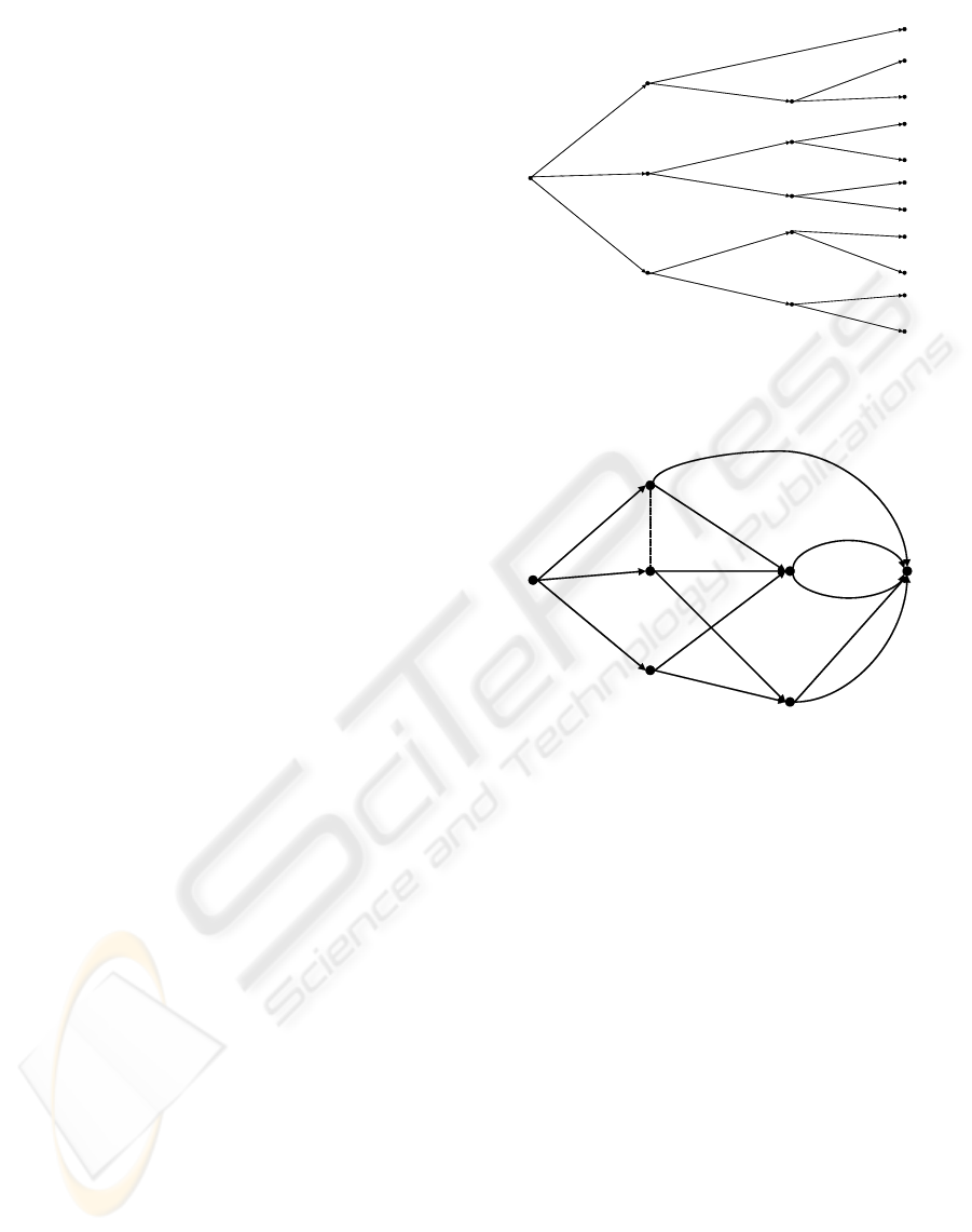
CEG-construction process is illustrated in Example 1,

and an example CEG in Figure 2.

Example 1

Consider the tree in Figure 1 which has 11 atoms

(root-to-leaf paths). Symmetries in the tree allow us

to store the distribution in 5 conditional tables which

contain 11 (6 free) probabilities. The transporter CEG

is produced by combining the vertices {v

, v

} into

one position w

, the vertices {v

, v

} into one position

, and all leaf-nodes into a single sink-node w

∞

. The

CEG C (Figure 2) has an undirected edge connecting

the positions w

and w

as these lie in the same stage –

their ﬂorets are topologically identical, and the edges

of these ﬂorets carry the same probabilities.

2 LEARNING CEGs

As the CEG can express a richer class of conditional

independence structures than the BN, CEG model se-

lection allows for the automatic identiﬁcation of more

subtle features of the data generating process than it

would be possible to express (and therefore to evalu-

ate) through the class of BNs. In this section we intro-

duce the techniques for learning CEGs and compare

them with those for learning BNs.

inf

Figure 1: Tree for Example 1.

inf

Figure 2: CEG for Example 1.

From our CEG deﬁnition, if w

, w

∈ u for some u,

then the corresponding edges in the ﬂorets F(w

)

and F(w

) carry the same probabilities. So, for

each member u of the set of stages prescribed by the

model under consideration for our CEG, we can la-

bel the edges leaving u by their probabilities under

this model. We can then let x

be the total number

of sample units passing through an edge labelled π

;

and the likelihood L(π

π) for our CEG model is given

L(π

π) =

∏

For BNs, the assumptions of local and global in-

dependence, and the use of Dirichlet priors ensures

conjugacy. The analogue for CEGs is to give the vec-

tors of probabilities associated with the stages inde-

pendent Dirichlet distributions. Then the structure of

the likelihood L(π

π) results in prior and posterior dis-

tributions for the CEG model which are products of

Dirichlet densities. The result of this conjugacy is

CHAIN EVENT GRAPH MAP MODEL SELECTION

393

that the marginal likelihood of each CEG is therefore

the product of the marginal likelihoods of its compo-

nent ﬂorets. Explicitly, the marginal likelihood of a

CEG C is

∏

Γ(

∑

)

Γ(

∑

(α

+ x

))

∏

Γ(α

+ x

)

Γ(α

)

where, as above

• u indexes the stages of C

• n indexes the outgoing edges of each stage

• α

are the exponents of our Dirichlet priors

• x

are the data counts

As we are actually interested in p(model | data),

and this is proportional to p(data | model) ×

p(model), we need to set both parameter priors and

prior probabilities for the possible models.

Exactly analogously with BNs, parameter modu-

larity in CEGs implies that whenever CEG models

share some aspect of their topology, we assign this as-

pect the same prior distribution in each model. When

such priors reﬂect our beliefs in a given context, this

can reduce our problem dramatically to one of sim-

ply expressing prior beliefs about the possible ﬂoret

distributions (ie. the local differences in model struc-

ture). As each CEG model is essentially a partition of

the vertices in the underlying tree into sets of stages,

this requirement ensures that when two partitions dif-

fer only in whether or not some subset of vertices be-

long to the same stage, the prior expressions for the

models differ only in the term relating to this stage.

The separation of the likelihood means that this local

difference property is retained in the posterior distri-

bution.

Now, our candidate set is much richer than the

corresponding candidate BN set, and will probably

contain models we have not previously considered in

our analysis. Again, evoking modularity, if we have

no information to suggest otherwise, we follow stan-

dard BN practice and let p(model) be constant for all

models in the class of CEGs. We now use the loga-

rithm of the marginal likelihood of a CEG model as

its score, and maximise this score over our set of can-

didate models to ﬁnd the MAP model.

Our expression has the nice property that the

difference in score between two models which are

identical except for a particular subset of ﬂorets, is

a function of the subscores only of the probabil-

ity tables on the ﬂorets where they differ. Vari-

ous fast deterministic and stochastic algorithms can

therefore be derived to search over the model space,

even when this is large – see (Freeman and Smith,

2009). This property is of course shared by the class

of BNs.

We set the priors of the hyperparameters so that

they correspond to counts of dummy units through the

graph. This can be done by setting a Dirichlet distri-

bution on the root-to-sink paths, and for simplicity we

choose a uniform distribution for this. It is then easy

to check that in the special case where the CEG is ex-

pressible as a BN, the CEG score above is equal to the

standard score for a BN using the usual prior settings

as recommended in, for example, (Cooper and Her-

skovits, 1992; Heckerman et al., 1995). As a compar-

ison with our CEG-expression; given Dirichlet priors

and a multivariate likelihood, the marginal likelihood

on a BN is expressible as

∏

i∈V

∏

Γ(

∑

imn

)

Γ(

∑

(α

imn

+ x

imn

))

∏

Γ(α

imn

+ x

imn

)

Γ(α

imn

)

where

• i indexes the set of variables of the BN

• n indexes the levels of the variable X

• m indexes vectors of levels of the parental vari-

ables of X

The importance of this result is that were we ﬁrst

to search the space of BNs for the MAP model, then

we could seamlessly reﬁne this model using the CEG

search score described above. Such embellishments

will allow us to search over models containing signif-

icant amounts of context speciﬁc information. Fur-

thermore any model we ﬁnd will have an associated

interpretation which can be stated in common lan-

guage, and can be discussed and critiqued by our

client/expert for its phenomenological plausibility.

Example 1 Continued

For the CEG in Figure 2, we put a uniform prior

over the 11 root-to-leaf paths, which in turn allows

us to assign our stage priors as follows: we assign

a Di(3, 4, 4) prior to the stage identiﬁed by w

, a

Di(3, 4) prior to the stage u

≡ (w

, w

), a Di(2, 2)

prior to each of the stages identiﬁed by w

and w

and a Di(3, 3) prior to the stage identiﬁed by w

. We

would then have a marginal likelihood of

KEOD 2009 - International Conference on Knowledge Engineering and Ontology Development

394

Γ(11)

Γ(11 + N)

Γ(3 + x

)Γ(4 + x

)

Γ(3)Γ(4)Γ(4)

Γ(7)

Γ(7 + x

+ x

)

Γ(3 + x

+ x

)Γ(4 + x

+ x

)

Γ(3)Γ(4)

Γ(4)

Γ(4 + x

)

Γ(2 + x

)Γ(2 + x

)

Γ(2)Γ(2)

Γ(6)

Γ(6 + x

+ x

)

Γ(3 + x

)Γ(3 + x

)

Γ(3)Γ(3)

Γ(4)

Γ(4 + x

+ x

)

Γ(2 + x

5·10

)Γ(2 + x

5·11

)

Γ(2)Γ(2)

where, with a slight abuse of notation, we let for ex-

ample x

be the data value associated with the edge

leaving w

labelled θ

; and where N is the sample size

∑

n=1

In this paper we have concentrated on the princi-

ple of assigning a score to a member of a candidate

class. For a more formal presentation of an algorithm

for searching over this class see (Freeman and Smith,

2009). An expanded version of this paper appears

at http://www2.warwick.ac.uk/fac/sci/statistics/

crism/research/2009/paper09-07, including an exam-

ple demonstrating the versatility of our method, and

an extended discussion section.

Note that the inputs to our search algorithm will

consist of a candidate set of models and data from the

problem we are modelling. The candidate set may be

constrained as described above. The output of the al-

gorithm will be the MAP model given the data and

our candidate set. As with learning BNs, exhaus-

tive search will be superexponential in the number of

problem variables. However, as with BNs for large

problems, fast local search algorithms can be devised

which quickly explore subclasses of CEGs that for

contextual reasons are expected to explain the data

well.

ACKNOWLEDGEMENTS

This research has been partly funded by the EPSRC

as part of the project Chain Event Graphs: Semantics

and Inference (grant no. EP/F036752/1).

REFERENCES

Cooper, G. F. and Herskovits, E. (1992). A Bayesian

method for the induction of Probabilistic Networks

from data. Machine Learning, 9(4):309–347.

Freeman, G. and Smith, J. Q. (2009). Bayesian model

selection of Chain Event Graphs. Research Report,

CRiSM.

Heckerman, D., Geiger, D., and Chickering, D. (1995).

Learning Bayesian Networks: The combination of

knowledge and statistical data. Machine Learning,

20:197–243.

Shafer, G. (1996). The Art of Causal Conjecture. MIT

Press.

Smith, J. Q. and Anderson, P. E. (2008). Conditional inde-

pendence and Chain Event Graphs. Artiﬁcial Intelli-

gence, 172:42–68.

Smith, J. Q., Riccomagno, E. M., and Thwaites, P. A.

(2009). Causal analysis with Chain Event Graphs.

Submitted to Artiﬁcial Intelligence.

Thwaites, P. A., Smith, J. Q., and Cowell, R. G. (2008).

Propagation using Chain Event Graphs. In Proceed-

ings of the 24th Conference on Uncertainty in Artiﬁ-

cial Intelligence, Helsinki.

CHAIN EVENT GRAPH MAP MODEL SELECTION

395