COMBINING TEMPORAL AND FREQUENCY BASED

PREDICTION FOR EEG SIGNALS

Padma Polash Paul, Howard Leung

Department of Computer Science, City University of Hong Kong, 83 Tat Chee Ave., Kowloon, Hong Kong

David A. Peterson

, Terrence J. Sejnowski

1,2

, Howard Poizner

Institute for Neural Computation, University of California, San Diego, U.S.A.

The Computational Neurobiology Lab, The Salk Institute, La Jolla, U.S.A.

Keywords: Electroencephalography, Temporal based Prediction, Frequency based Prediction, Artificial Neural

Network.

Abstract: This paper presents a novel approach for electroencephalogram (EEG) signal prediction. It combines

temporal and frequency based prediction to achieve a good final prediction result. Artificial neural networks

are used as the predictive model for signals both in the temporal and frequency domain. In frequency based

prediction, the amplitude and the phase of the frequency response are predicted separately. Experiments

were conducted on the prediction of EEG data recorded from 13 subjects. Eight performance measures were

used to evaluate the performance of our proposed method. Experiment results show that the proposed

combined prediction method gives the overall best performance compared with the temporal based

prediction alone and the frequency based prediction alone.

1 INTRODUCTION

Time series prediction problem has wide range of

research interest due to its diverse potential

applications such as electroencephalogram (EEG)

signal analysis, financial data prediction, and

environmental monitoring. To measure brain

activity, non-invasive EEG is one of the most

important bio-signals and many researchers are

working on EEG signal prediction.

Researchers have used time series prediction

methods to check the linearity of EEG signals. They

found that nonlinear properties are present in EEG

signals and that some data are not predictable using

linear stochastic system (Robert A. Stêpieñ, 2002). It

was found that EEG recordings from subjects with

schizophrenia contain some degree of determinism

(low order chaotic), but are not completely

deterministic and contain properties of nonlinearity

(Ying-Jie Li, 2005). The linear EEG model cannot

perfectly describe the spontaneous EEG that

displays nonlinear phenomena (Ou Bai, 2000).

Time series prediction methods were also

applied to find the occurrence of seizures from the

EEG of epilepsy patients (Florian Mormann, 2007).

EEG time series prediction also has been used to

extract features for motor imagery task classification

in Brain Computer Interfaces (Stefan Cososchi,

2006). EEG time series prediction pre-processing

shows better performance compared with Common

Spatial Pattern (Damien Coyle, 2008). From

previous research, it is clear that EEG time series

prediction has a high impact on medical and

engineering applications.

Different algorithms for EEG signal prediction

have been proposed to enhance the predictive

model’s convergence performance in the time

domain, such as Least Square Support Vector

Machine (LS-SVM), Support Vector Regression

(SVR), Neuro-Fuzzy System, recurrent or time delay

network, and feature selection methods such as

mutual information based feature selection.

(Nicholas I., 2009) Researchers also combine

Principal Component Analysis (PCA) (Paul Cristea,

2008), Kernel PCA and SVM (Qisong Chen, 2008),

Independent Component Analysis (ICA) (Juan M.

Gorriz, 2003), for feature selection purpose in the

time domain. Future EEG signal prediction is

Polash Paul P., Leung H., A. Peterson D., J. Sejnowski T. and Poizner H. (2010).

COMBINING TEMPORAL AND FREQUENCY BASED PREDICTION FOR EEG SIGNALS.

In Proceedings of the Third International Conference on Bio-inspired Systems and Signal Processing, pages 29-36

DOI: 10.5220/0002696800290036

 SciTePress

necessary to predict the future brain activity in

which users may have different stages of intention.

In this work, the EEG to be predicted is recorded

during a time in which tasks conditions are

changing. At some points in time, subjects

are responding to rewards or making decisions,

making movements, or doing none of these things.

To predict the EEG would be related to what task

conditions the subject was performing at particular

points in the prediction interval.

For nonlinear time series prediction, the future

to some extent may be predicted, but the accuracy of

the non-linear forecast falls off with increasing

intervals of prediction time for uncorrelated noise

(K.J. Blinowska, 1991). On the other hand, the EEG

reflects thousands of simultaneous ongoing brain

processes. The brain’s response to a single stimulus

or event of interest is not usually visible in the EEG

recording of a single trial. To see the brain response

to the stimulus, many trials are typically averaged

(Coles, 1996).

We propose a method for EEG signal prediction

that combines temporal and frequency based

prediction. In our problem, a segment of future EEG

signals is predicted given some known values of the

EEG signal in the past. Using only time domain

data, prediction causes high prediction error for

noise and for the model error. On the other hand,

brain activities such as internal and external

cognitive processing have great impact on particular

frequency bands. This provides good motivation to

perform the prediction in the frequency domain. The

prediction from the temporal domain and the one

from the frequency domain are combined by

considering their performance in the training data.

The remainder of the paper is organized as

follows. The proposed method is described in

Section 2. Experiments and results are provided in

Section 3. The conclusions and future work are

stated in Section 4.

2 PROPOSED METHOD

2.1 Input Data Representation

Time series prediction is a well known problem for

forecasting future value. One-step-ahead time series

prediction can be presented by Equation (1):

),(

yyyy

Ltttt

−−−

= "

(1)

where y

is predicted based on the past L values in

the time series.

For future brain activity or event prediction

segments of multiple time samples are predicted. As

illustrated in Figure 1, the time segment Y

containing M sample points is predicted based on N

sample points in the past.

Figure 1: A time segment with M sample points to be

predicted from N known sample points.

2.2 Overview of the Proposed System

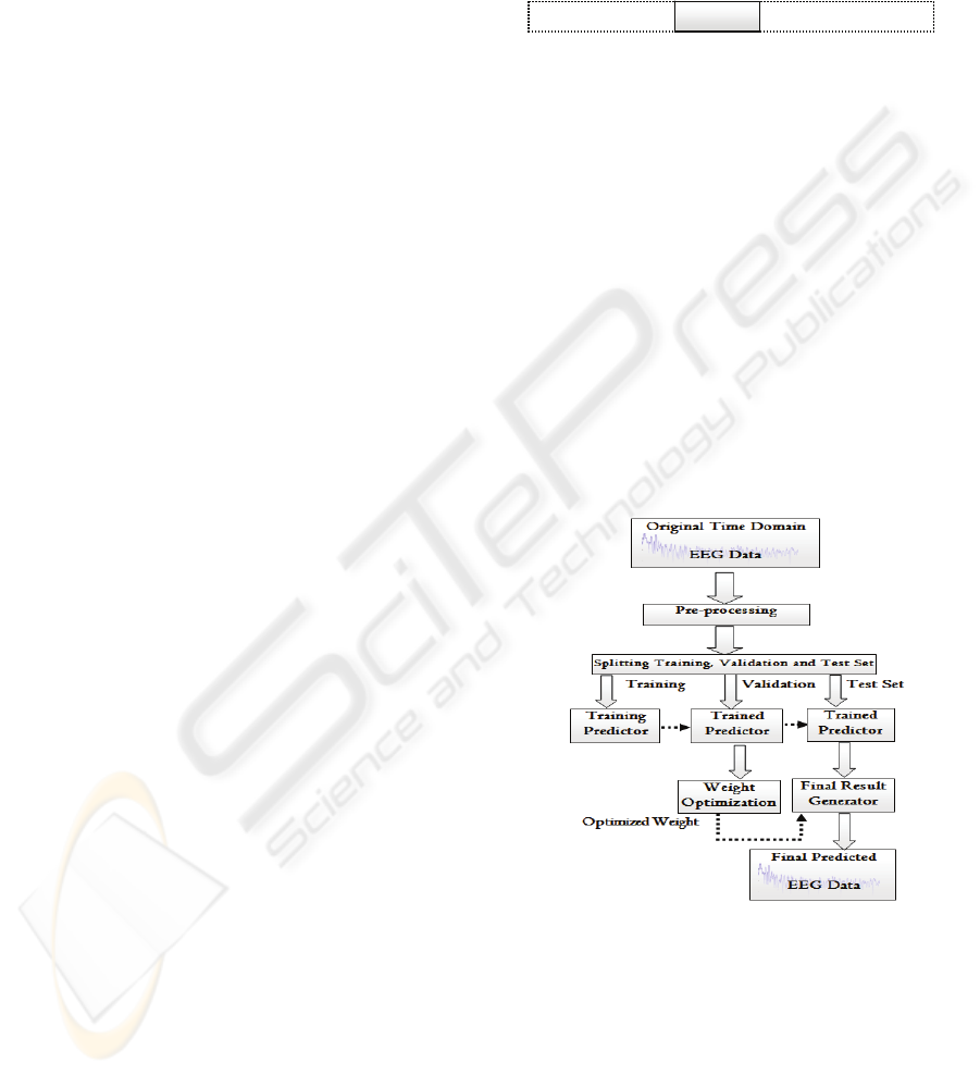
Figure 2 presents a block diagram of the prediction

process. After preprocessing, the EEG data are

divided into training, validation and test sets. The

trained predictor is then validated using the

validation data set. Different predictors are trained

for the temporal based prediction and the frequency

based prediction separately. The resulting

predictions are then combined using weights that

optimize the results in the training data. Based on

the validation performance, a set of weights is

selected and used to generate the final result in the

testing process.

Figure 2: Block diagram of the prediction system.

The following sections explain each of the

system modules in more detail.

2.3 Pre-processing

The raw EEG data are normalized by rescaling the

signal to the range [0,1] to meet the high

convergence in the neural network based training

1 2 3 .... N N+1 ... N+M N+1+M ...

... ... ... y

BIOSIGNALS 2010 - International Conference on Bio-inspired Systems and Signal Processing

process. This pre-processing step is illustrated by

Equation (2):

minmax

min

−

(2)

2.4 Proposed Prediction Algorithm

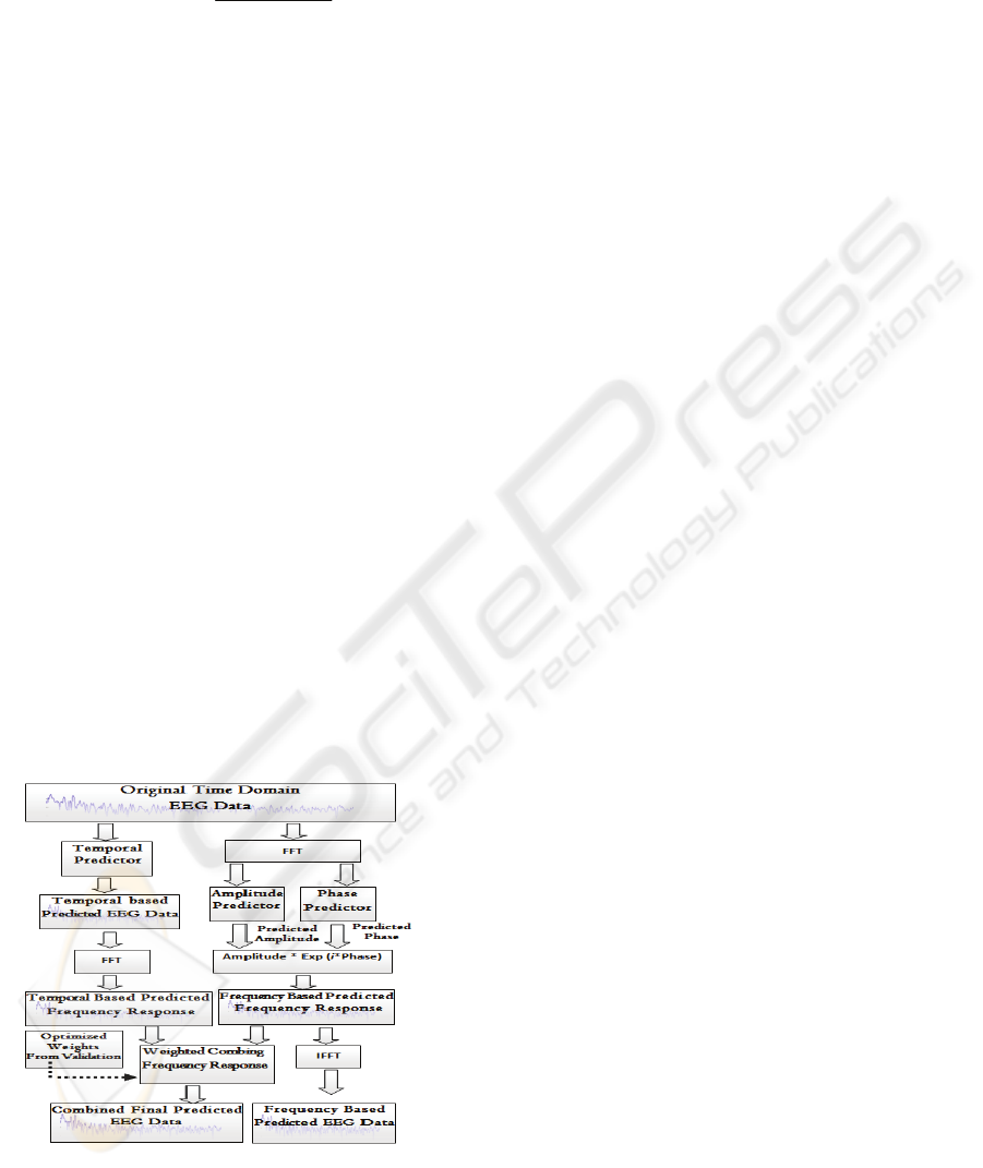
Figure 3 shows the workflow of our proposed

prediction algorithm. Our proposed prediction

algorithm is divided into two main steps. In the first

step, the temporal domain data and its corresponding

frequency domain data are predicted separately. In

the frequency based prediction, Fast Fourier

Transformation is used to convert the time signal

into the frequency domain. From the frequency

response data, the amplitude and the phase are

computed. Two neural networks are built to predict

the amplitude and the phase separately. In Figure 3,

these predictors are shown in two blocks named

Amplitude Predictor and Phase Predictor. The

predicted frequency response data are reconstructed

using the predicted amplitude and the predicted

phase as shown in Equation (3).

)(

)()(

tphasei

etamplitudetf

×=

(3)

Inverse Fast Fourier Transformation is applied to get

the frequency based predicted data in time domain.

In the second step, the temporal and frequency

based predicted data are combined by using weights

obtained from the analysis of the prediction error for

each frequency band of each predicted signal during

the validation process.

Figure 3: Workflow of the proposed prediction algorithm.

2.5 Predictive Model

The Neural Network parameters are obtained using a

two fold cross validation process. For the temporal

and frequency based predictions, gradient descent

with momentum and adaptive learning rate back-

propagation is used. Parameters are optimized

separately to get the best performance in each

domain. Learning rate in the range 0.01-0.03 and

momentum of 0.3-0.9 gives better performance.

Iteration range is 2000-2500 to train the predictor. A

three layered back-propagation neural network is

used for the system. The number of the input and

output nodes are equal to the known segment length

and predicted segment length respectively. The

number of hidden nodes is optimized both in

temporal and frequency domain. The number

optimized hidden nodes are in the range of 36-120.

Log-sigmoid functions are used as transformation

function.

Our proposed prediction algorithm is a general

framework and it can work regardless of the

predictive model to be applied. The proposed

method is checked with the gradient decent learning

without momentum and the overall performance is

lower than the case of gradient decent with

momentum. The neural network parameters such as

the value of momentum and transformation function

are varied and it is found that the performance is

very similar with negligible difference.

2.6 Weighted Combining

From the predicted results of the temporal and

frequency domains, the weights are optimized from

the validation set. There are two possible ways to

combine the temporal and frequency based predicted

data: 1) in frequency domain and 2) in time domain.

Combining in the frequency domain has the

advantage of being able to put more emphasis in a

particular frequency band if the corresponding

prediction signal is shown to be more accurate. Next

we will show how we calculate the weights.

Figure 4 illustrates the process for computing the

weights used to combine the temporal-based

predicted frequency response and the frequency-

based predicted frequency response. Each frequency

response is divided into n frequency bands. The

frequency bands FRt

,FRt

......

,FRt

represent the

frequency response of the signal predicted in the

temporal domain. The frequency bands

FRf

,FRf

......

,FRf

represent the frequency response

of the signal predicted in the frequency domain.

With the validation set, the ground truth frequency

COMBINING TEMPORAL AND FREQUENCY BASED PREDICTION FOR EEG SIGNALS

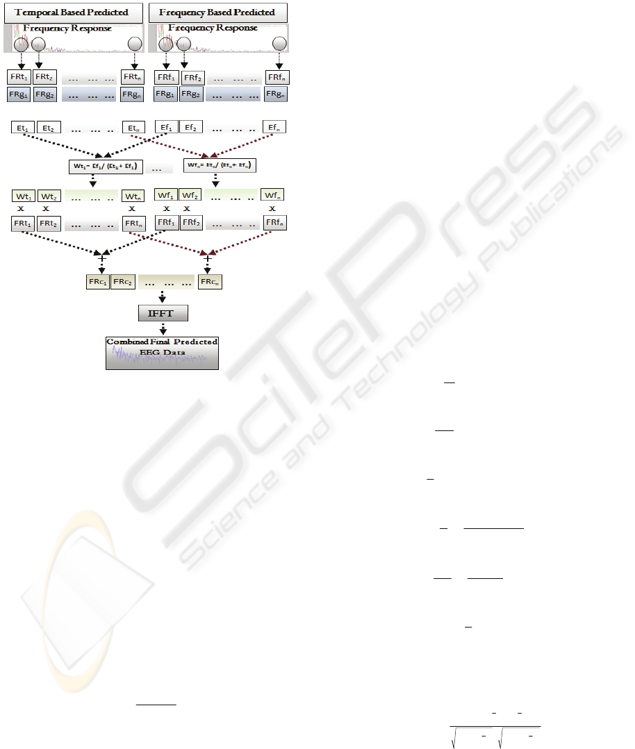
response FRg

,FRg

......

,FRg

of the actual signal is

known. During the validation, this ground truth

information is compared with the prediction from

the temporal domain and the prediction from the

frequency domain at each frequency band.

Figure 4: Weight calculation and the combining process of

predicted frequency response data.

Errors are then computed in order to determine

how good the prediction is in each domain. The

error E

denotes the error between the i-th frequency

band of the temporal based predicted frequency

response and that of the ground truth frequency

response. Similarly, the error E

denotes the error

between the i-th frequency band of the frequency

based predicted frequency response and that of the

ground truth frequency response. The smaller the

error is, the better the corresponding prediction is.

The weights for combining the temporal based

predicted frequency response and the frequency

based predicted frequency response for the i-th

frequency band are denoted by W

and W

respectively. These weights are calculated by

Equations (4) and (5):

fiti

(4)

tifi

−

(5)

It can be seen from Equations (4) and (5) that if

the error for a particular prediction method is small

at a frequency band, then the corresponding weight

will be set to be higher. For example, if temporal

based prediction yields a small error E

, then this

means that the error from the frequency based

prediction E

is relatively larger. From Equations (4)

and (5), it can be observed that the weight W

will

become larger than the W

thus putting more

emphasis on the temporal based prediction.

After calculating the weights, the corresponding

frequency bands are then multiplied and added to get

the combine frequency band FRc

,FRc

......

,FRc

Inverse Fourier Transformation is used to transform

the combined response back to the time domain

signal.

2.7 Performance Measures

Eight different performance measures are used to

check the system performance. These performance

measures are defined by Equations (6)-(13). For the

first five measures MSE, NMSE, MAE, NMAE,

MAPE, the larger the values are, the worse the

performance is. For the last three measures SNR,

PSNR, CCORR, the larger the values are, the better

the performance is.

 Mean Square Error (MSE)

)y(y

MSE

−=

∑

(6)

 Normalized Mean Square Error (NMSE)

)y(y

nσ

NMSE

−=

∑

(7)

 Mean Absolute Error (MAE)

y|y

MAE −=

∑

(8)

 Normalized Mean Absolute Error (NMAE)

∑

−

)y(y

|y|y

NMAE

minmax

(9)

 Mean Absolute Percentage Error (MAPE)

∑

−

||y

|y|y

MAPE

100

(10)

 Signal-to-Noise Ratio (SNR)

/MSE)y

(SNR

∑

log10

(11)

 Peak Signal-to-Noise Ratio (PSNR)

/MSE)

peak

(yPSNR

log10=

(12)

 Cross Correlation (CCORR)

∑∑

∑

−×−

)y(y)x(x

CCORR

(13)

BIOSIGNALS 2010 - International Conference on Bio-inspired Systems and Signal Processing

2.8 Effect of Weight on Performance

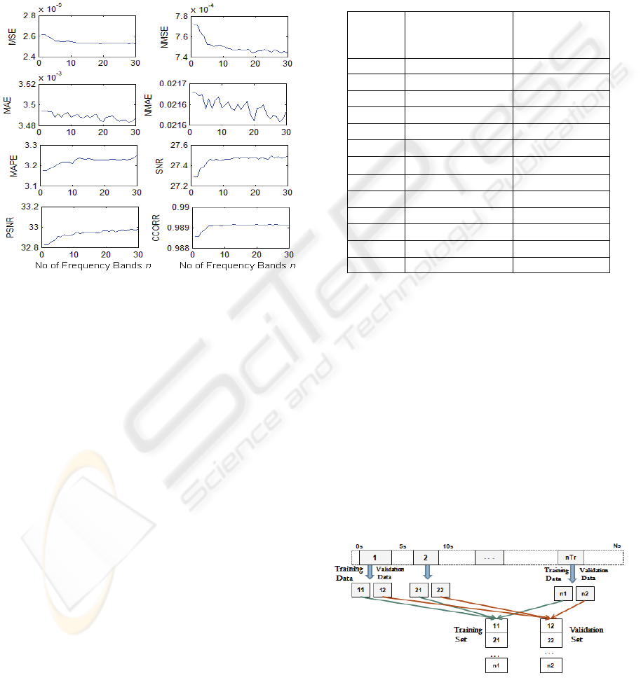
We examine how the performance is affected by the

number of frequency bands n considered. Figure 5

shows the effect of number of frequency bands on

the performance with different error measures. From

the analysis of the results, we found that for all

performance measures if the number of frequency

bands increases then the performance also increases.

Figure 5: Performance with different number of frequency

bands n.

3 EXPERIMENT AND RESULTS

3.1 Data Acquisition

The EEG signals were collected with a Biosemi

EEG system with 10/20 international standard

(http://www.biosemi.com) from a total of 13 young

adult subjects. The sampling frequency (f

) was

512Hz. The behavioural task was an instrumental

reward-based learning task adapted for humans

(Peterson et al., 2009), based on a primate study

designed to examine the firing rates of dopamine

cells during decision making (Morris et al., 2006).

The task is a modification of the classic two-armed

bandit (Robbins, 1952). Subjects were presented

with a series of trials in which they chose abstract

visual images with a possibility of accruing a small

reward on each trial. The task consists of two phases

of 256 trials of reference and decision. Subjects were

first given a brief practice session, with eight

reference and four decision trials. The practice

stimuli were four simple geometric shapes that were

different from any of the stimuli used in the actual

experiment. There were no feedback signals or

rewards in this practice session in order to avoid

teaching any associations prior to the actual

experiment. Table 1 shows the number of sample

points as well as the total time in second in which

the EEG signal for each of the 13 subjects is

recorded.

Table 1: Number of sample points and time in EEG

recoding for the subjects.

Subject Number of

Sample Points

=512Hz)

Time (second)

1 1285120 2510

2 1126400 2200

3 949760 1855

4 1172480 2290

5 1246720 2435

6 1141760 2230

1077760 2105

8 1100800 2150

9 1226240 2395

10 1044480 2040

11 1231360 2405

12 1044480 2040

13 1008640 1970

3.2 Data Preparation

The data for each subject are segmented into

different sections as shown in Figure 6. Each section

is further divided into two equal subsections, one

used for training and the other used for validation

purpose.

The unused portions of the data shown in Figure

6 are used to for testing. Figure 7 illusrates the test

set generation for a subject.

After splitting the data for a subject, the training sets

are processed for input into the predictive model

(Neural Network in our case). Based on the N

known sample points, M sample points are to be

predicted.

Figure 6: Training and validation set spliting for a subject.

COMBINING TEMPORAL AND FREQUENCY BASED PREDICTION FOR EEG SIGNALS

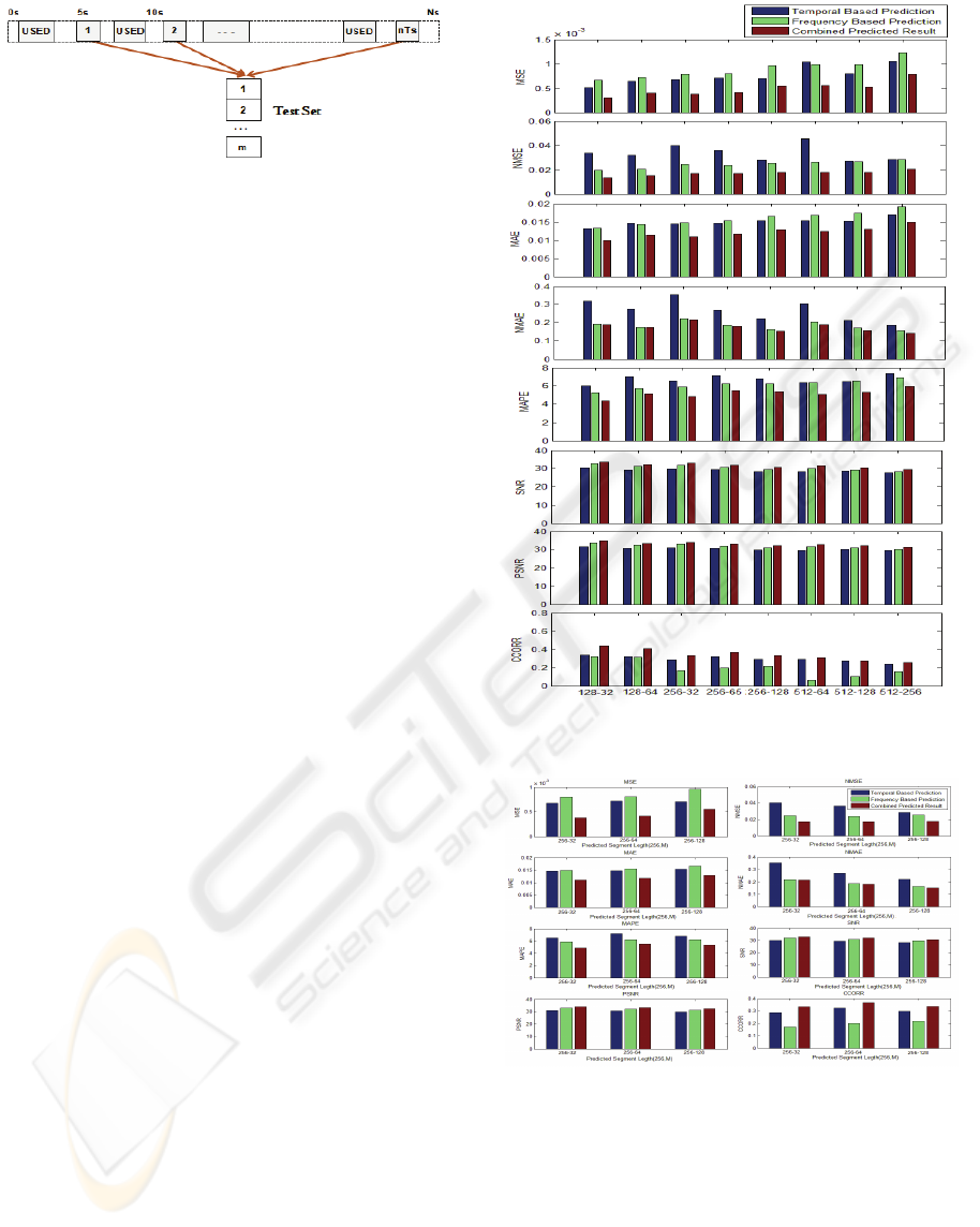
Figure 7: Test set genaration for a subject.

Eight different pairs of parameters (N, M) are

used to check the performance of the proposed

method: (128, 32), (128, 64), (256, 32), (256, 64),

(256, 128), (512, 64), (512, 128), (512, 256).

3.3 Results

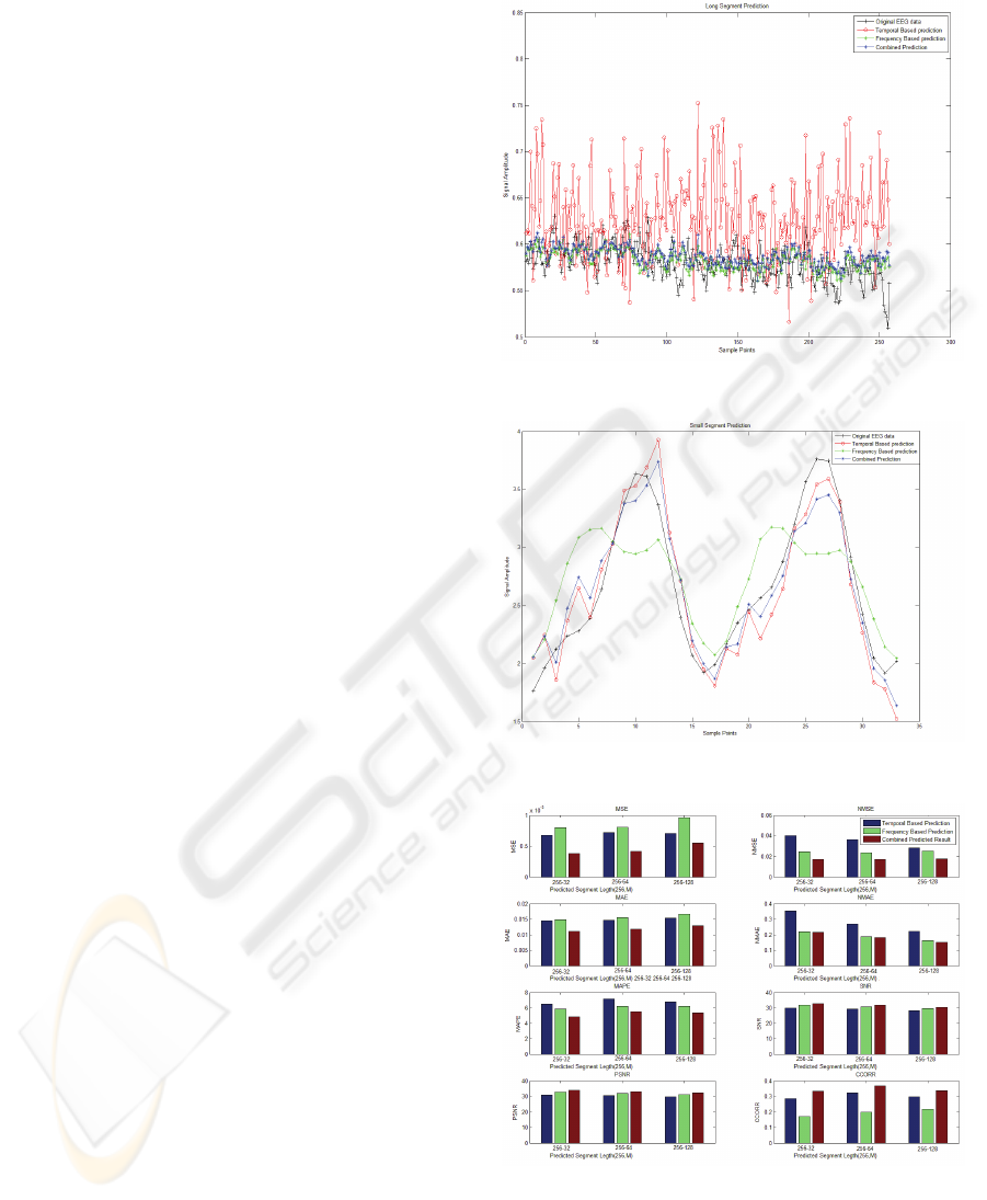
The performance averaged over all subjects with

different values of (N, M) using our proposed

method is shown in Figure 8. Temporal based

prediction performance is better than the frequency

based prediction for MSE, MAE, SNR and CCORR.

On the other hand, frequency based prediction gives

better performance for NMSE, NMAE, MAPE, and

PSNR. It can be seen from Figure 8 that the case

with N=128 and M=32 gives the best average result.

It can also be observed that the performance

degrades when the number of samples to be

predicted becomes larger, i.e., when M is larger. An

example prediction with a large value of M=256 is

shown in Figure 11 (Appendix). Another example

prediction with a small value of M=32 is shown in

Figure 12 (Appendix).

Figure 9 compares the performance with

different values of M (M=32, 64, 128) at a fixed

value of N=256. From the analysis of the results, we

found that for long segments, frequency based

prediction gives better performance than temporal

based prediction. For example, with the measures

NMSE, NMAE and CCORR, frequency based

prediction gives better performance with N=256 and

M=128. With the measures MSE and MAE,

temporal based prediction gives better performance

in this case. The other three measures SNR, PSNR

and MAPE give similar performance in both

temporal and frequency based prediction. Similar

results are found from the analysis of the cases

(N=512 and M=64, 128, 256) shown in Figure 13

(Appendix).

Figure 10 shows the performance averaged

among all subjects and among all the 8 parameter

pairs of (N, M).

Figure 8: Performance averaged among all subjects under

different values of N-M shown in the x-axis.

Figure 9: Performance comparison for different values of

M at a fixed value of N=256.

It can be observed from Figure 10 that the

performance of proposed combined prediction

approach is better than the performance with the

temporal based prediction or the frequency based

prediction alone with all the 8 measures. Frequency

based prediction gives better performance than

temporal based prediction for the performance

measures NMSE, MAPE, NMAE, SNR and PSNR.

BIOSIGNALS 2010 - International Conference on Bio-inspired Systems and Signal Processing

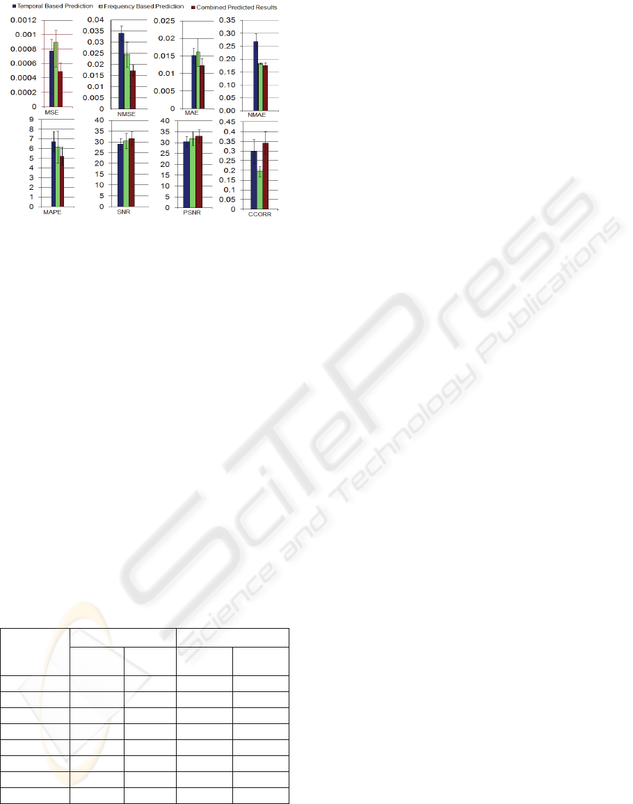
Figure 10: Performance averaged over all subjects and all

parameter pairs (N, M).

For the other three measures MSE, MAE and

CCORR, temporal based prediction gives better

performance than frequency based prediction.

3.4 Statistical Test

The t-tests (one tailed and paired) were performed to

test the statistical significance of the final results of

the eight different performance measures. We tested

the significance of differences between S

-S

and

-S

pairs, where S

, S

and S

are performance

of all subjects in temporal, frequency and combined

domain based prediction results, respectively. The

differences in test scores had approximately normal

distributions. A significance level of α=0.1 was

used. Table 2 shows the t-values and p-values for

different performance measures. We have accepted

most of the measures, because in most of the cases

p<0.1. Subscript of error measures R and L

represent right and left tailed test respectively.

Table 2: Statistical t-Test Result.

Error

Measure

t-Value

(df=12)

p-Values

-S

MSE

3.037

1.502 0.0052 0.0794

NMSE

5.003

1.662 0.0002 0.0611

MAE

6.003

1.647 0.0000 0.0628

NMAE

4.191

0.629 0.0006 0.2706

MAPE

4.611

0.935 0.0003 0.1841

SNR

4.429

1.612 0.0004 0.0665

PSNR

4.427

1.612 0.0004 0.0665

CCORR

3.103

3.422 0.0046 0.0025

4 CONCLUSIONS AND FUTURE

WORK

In this paper, we propose a method for predicting

time series data. Our approach works by combining

temporal based prediction and frequency based

prediction. We apply our proposed method to the

prediction of EEG signals recorded from 13

subjects. From the experiments, it is found that

frequency based prediction gives better performance

than the temporal prediction and that the combined

final result gives the best performance. In our

experiments, eight different performance measures

were used to evaluate the performance since

different performance measure may be preferred in

different applications.

In future studies, we will apply the system to

predict future brain activity, future user intention for

decision-making and arm movements in an

instrumental reward-based learning task. We will

also use different methods of signal decomposition

to acheive better prediction performance.

ACKNOWLEDGEMENTS

The work described in this paper was fully

supported by a grant from the Research Grants

Councils of the Hong Kong Special Administration

Region, China (Project No. CityU 1165/09E), and

by NSF grant #SBE-0542013 to the Temporal

Dynamics of Learning Center, an NSF Science of

Learning Center.

REFERENCES

Peterson, D.A.,

Elliott, C., Song, D.D., Makeig, S.,

Sejnowski, T.J., Poizner, H. Probabilistic reversal

learning is impaired in Parkinson’s disease,

Neuroscience, July 20, 2009 [E-pub ahead of print].

G., Morris, Alon N., David A., E., Vaadia1, H.,

Bergman, 2006. Midbrain dopamine neurons encode

decisions for future action. Nature Neuroscience.

Volume 9.

H. Robbins, 1952. Some aspects of the sequential design

of experiments. Bulletin of the American

Mathematical Society.

Robert A. Stêpieñ, 2002. Testing for non-linearity in EEG

signal of healthy subjects. Acta Neurobiol. Exp.

Ying-Jie Li, Yi-Sheng Zhu, and Fei-Yan Fan, 2005.

Detecting the Determinism of EEG Time Series Using

a Nonlinear Forecasting Method. IEEE Engineering in

Medicine and Biology 27th Annual Conference.

Shanghai, China.

COMBINING TEMPORAL AND FREQUENCY BASED PREDICTION FOR EEG SIGNALS

Florian Mormann, Ralph G. Andrzejak, Christian E. Elger

and Klaus Lehnertz, 2007. Seizure prediction: the long

and winding road. Brain, Published by Oxford

University Press on behalf of the Guarantors of Brain.

Damien Coyle1, Girijesh Prasad2 and Thomas M.

McGinnity, 2004. Extracting Features for a Brain-

Computer Interface by Self-Organising Fuzzy Neural

Network-based Time Series Prediction. Proceedings of

the 26th Annual International Conference of the IEEE

EMBS San Francisco, CA, USA.

Damien Coyle, Abdul Satti, Girijes Prasad, Thomas M.

McGinnity, 2008. Neural Time-Series Prediction Pre-

processing Meets Common Spatial Patterns in Brain-

Computer Interface. 30

Annual International

Conference Vancouver, British Columbia, Canada, pp.

2626-2629.

Nicholas I., Sapankevych, 2009. Time Series Prediction

Using Support Vector Machines: A Survey. IEEE

Computational Intelligence Magazine. pp.25-38

Paul Cristea, V., mladenov, G., Tsenov, Rodica T.,

Simona P., 2008. Application of neural network, PCA

and feature extraction for prediction of nucleotide

sequence by using genomic signals. 9

Symposium on

Neural Network Application in Electrical Engineering,

NEURAL-2008.

Qisong Chen, Xiaowei Chen, Yun Wu, 2008. The

Combining Kernel Principal Component Analysis with

Support Vector Machine for Time Series Prediction

Model. 2

International Symposium of Inteligent

Information Technology. pp. 90-94

K.J. Blinowska and M. Malinowski, 1991. Non-linear and

linear forecasting of the EEG time series. Biological

Cybernetics, Springer-Vcrlag.

Coles, Michael G.H., Michael D. Rugg, 1996. "Event-

related brain potentials: an introduction".

Electrophysiology of Mind. Oxford Scholarship Online

Monographs.

http://www.biosemi.com

Ou Bai, M., Nakamura, Akio Ikeda, Hiroshi Shibasaki,

2000. Nonlinear Markov Process Amplitude EEG

Model for Nonlinear Coupling Interaction of

Spontaneous EEG. IEEE Transaction on Biomedicine

Engineering, VOL. 47, NO. 9.

J.M.Gorriz, C.G.Puntonet, M. Salmeron, E.W. Lang, Time

series prediction using ICA algorithms", Proceedings

of the Second IEEE International Workshop on

Intelligent Data Acquisition and Advanced Computing

Systems: Technology and Applications, pp. 226-230,

2003

APPENDIX

Figure 11: Prediction result of a longer segment (M=256) .

Figure 12: Prediction result of a shorter segment (M=32) .

Figure 13: Performance comparison for different values of

M at a fixed value of N=512.

BIOSIGNALS 2010 - International Conference on Bio-inspired Systems and Signal Processing