
LEARNING ACTION SELECTION STRATEGIES IN COMPLEX
SOCIAL SYSTEMS
Marco Remondino, Anna Maria Bruno and Nicola Miglietta
Management and Administration Department, University of Turin, Italy
Keywords: Management, Action selection, Reinforcement learning.
Abstract: In this work, a new method for cognitive action selection is formally introduced, keeping into consideration
an individual bias for the agents: ego biased learning. It allows the agents to adapt their behaviour accord-
ing to a payoff coming from the action they performed at time t-1, by converting an action pattern into a
synthetic value, updated at each time, but keeping into account their individual preferences towards specific
actions. In agent based simulations, the many entities involved usually deal with an action selection based
on the reactive paradigm: they usually feature embedded strategies to be used according to the stimuli com-
ing from the environment or other entities. The actors involved in real Social Systems have a local vision
and usually can only see their own actions or neighbours’ ones (bounded rationality) and sometimes they
could be biased towards a particular behaviour, even if not optimal for a certain situation. Some simulations
are run, in order to show the effects of biases, when dealing with an heterogeneous population of agents.
1 INTRODUCTION
Multi agent models allow to capture the complexity
by modeling the system from the bottom, by defin-
ing the agents’ behavior and the rules of interaction
among them and the environment. Agent Based Si-
mulation (ABS), in this field, is not only about un-
derstanding the individual behavior of agents, or in
optimizing the interaction among them, in order to
coordinate their actions to reach a common goal, like
in other Multi Agent Systems (MAS), but above all
it’s about re-creating a real social system (e.g.: a
market, an enterprise, a biological system) in order
to analyze it as if it were a virtual laboratory for ex-
periments. Reactive agents or cognitive ones can be
employed in multi agent systems (Remondino,
2005); while the former model deals with the stimu-
lus-reaction paradigm, the latter provides a “mind”
for the agents, that can decide which action to take at
the next step, based on their previous actions and the
state of the world. When dealing with the problem of
action selection, reactive agents simply feature a
wired behavior, deriving from some conditional em-
bedded rules that cannot be changed by the circums-
tances, and must be foreseen and wired into them by
the model designer. For example given a set of
agent’s states
,
, and a set of agent’s actions
,
, a deterministic reactive agent could con-
sist of a set of rules like:
;
(1)
Or, if we have a wider set of states
,…,
,
with , but again just a binary set of actions to
be performed
,
, the rule could be as follows:
,
;
(2)
Where “range” is used to synthetically indicate the
states among 1 and k, in the system. This can be ap-
plied in the same way with several discrete intervals,
instead of just two. Of course, if the actions are more
than two, like a set
,…,
, the rules can be
simply multiplied as follows:
…
(3)
And linear combinations of both sets. The state
of the agent could be function of both a stimulus
coming from the environment and of some action
performed by other agents or by the agent itself.
Reactive agents could also be stochastic, in the
sense that they could have a probabilistic distribu-
tion connected to their action selection function. For
each action/state combination a probability function
274
Remondino M., Maria Bruno A. and Miglietta N. (2010).
LEARNING ACTION SELECTION STRATEGIES IN COMPLEX SOCIAL SYSTEMS.
In Proceedings of the 2nd International Conference on Agents and Artificial Intelligence - Agents, pages 274-281
DOI: 10.5220/0002706802740281
Copyright
c
SciTePress

is defined, so that for a defined
and a de-
fined
we have that:
,
where 01
(4)
And
,
1
(5)
As an example we may think of a simple situa-
tion in which we have two possible actions
,
so
that for a particular state
we could have that
,
0.2 and that
,
0.8, meaning
that the agent, when facing the state
will perform
20% of the times the action
and 80% of the times
action
, using a uniform distribution.
Some actions could feature a probability of 0 for
certain states, and others could have a probability of
1 for a given state. If all the probabilities for the ac-
tions, given a state, are either 0 or 1, we are back at
the deterministic situation presented above since, in
that particular case, only one action could be per-
formed (probability equal to 1) while the others
would never be performed (probability equal to 0).
Reactive agents can be good for simulations,
since the results obtained by employing them are
usually easily readable and comparable (especially
for ceteris paribus analysis). Besides, when the
agent’s behavior is not the primary focus, reactive
agents, if their rules are properly chosen, can give
very interesting aggregate results, often letting
emergent system properties emerge at a macro level.
Though, in situations in which, for example, learn-
ing coordination is important, or the focus is on ex-
ploring different behaviors in order to dynamically
choose the best one for a given state, or simply
agent’s behavior is the principal topic of the re-
search, cognitive agents could be employed, embed-
ded with some learning technique. Besides, if the
rules of a reactive agent are not chosen properly,
they could bias the results; these rules, in fact, are
chosen by the designer and could thus reflect her
own opinions about the modeled system. Since
many ABS of social systems can formulated as stage
games with simultaneous moves made by the agents,
some learning techniques derived from this field can
be embedded into them, in order to create more rea-
listic response to the external stimuli, by endowing
the agents with a self adapting ability. Though, mul-
ti-agent learning is more challenging than single-
agent, because of two complementary reasons.
Treating the multiple agents as a single agent in-
creases the state and action spaces exponentially and
is thus unusable in multi agent simulation, where so
many entities act at the same time. On the other
hand, treating the other agents as part of the envi-
ronment makes the environment non-stationary and
non-Markovian (Mataric, 1997). In particular, ABS
are non-Markovian systems if seen from the point of
view of the agents (since the new state is not only
function of the individual agent’s action, but of the
aggregate actions of all the agents) and thus tradi-
tional Q-learning algorithms (Watkins, 1989; Sutton
and Barto, 1998) cannot be used effectively: the ac-
tors involved in real Social Systems have a local vi-
sion and usually can only see their own actions or
neighbours’ ones (bounded rationality) and, above
all, the resulting state is function of the aggregate
behaviours, and not of the individual ones.
While, as discussed in Powers and Shoham
(2005), in iterated games learning is derived from
facing the same opponent (or another one, with the
same goals), in social systems the subjects can be
different and the payoff could not be a deterministic
or stochastic value coming from a payoff matrix.
More realistically, in social systems the payoff could
be a value coming from the dynamics of interaction
among many entities and the environment, and could
have different values, not necessarily within a pre-
defined scale. Besides, social models are not all and
only about coordination, like iterated games, and
agents could have a bias towards a particular beha-
vior, preferring it even if that’s not the best of the
possible ones. An example from the real world could
be the adoption of a technological innovation in a
company: even though it can be good for the enter-
prise to adopt it, the managerial board could be bi-
ased and could have a bad attitude towards technol-
ogy, perceiving a risk which is higher than the real
one. Thus, even by looking at the positive figures
coming from market studies and so on, they could
decide not to adopt it. This is something which is not
taken into consideration by traditional learning me-
thods, but that should be considered in ABS of so-
cial systems, where agents are often supposed to
mimic some human behavior. Besides, when the
agents are connected through a social network, the
experience behind a specific action could be shared
with others, and factors like the individual reputation
of other agents could be an important bias to indi-
vidual perception. In order to introduce these factors,
a formal method is presented in the paper: Ego Bi-
ased Learning (EBL). Another paradigm is briefly
described as a future development, called Reputation
Based Socially Biased Learning.
The purpose of this work is not that of supplying
an optimized algorithm for reinforcement learning
(RL); instead, the presented formalisms mimic as
much as possible the real cognitive process taken by
human agents involved in a social complex system,
when needing to take an individual strategic deci-
sion; this is useful to study aggregate results.
LEARNING ACTION SELECTION STRATEGIES IN COMPLEX SOCIAL SYSTEMS
275

2 REINFORCEMENT LEARNING
Learning from reinforcements has received substan-
tial attention as a mechanism for robots and other
computer systems to learn tasks without external su-
pervision.
The agent typically receives a positive payoff from
the environment after it achieves a particular goal,
or, even simpler, when a performed action gives
good results. In the same way, it receives a negative
(or null) payoff when the action (or set of actions)
performed brings to a failure. By performing many
actions overtime (trial and error technique), the
agents can compute the expected values (EV) for
each action. According to Sutton and Barto (1998)
this paradigm turns values into behavioral patterns;
in fact, each time an action will need to be per-
formed, its EV, will be considered and compared
with the EVs of other possible actions, thus deter-
mining the agent’s behavior, which is not wired into
the agent itself, but self adapting to the system in
which it operates.
Most RL algorithms are about coordination in multi
agents systems, defined as the ability of two or more
agents to jointly reach a consensus over which ac-
tions to perform in an environment. In these cases,
an algorithm derived from the classic Q-Learning
technique (Watkins, 1989) can be used. The EV for
an action –
– is simply updated every time the
action is performed, according to the following, re-
ported by Kapetanakis and Kundenko (2004):
(6)
Where 01 is the learning rate and p is the
payoff received every time that action a is per-
formed.
This is particularly suitable for simulating multi
stage games (Fudenberg and Levine 1998), in which
agents must coordinate to get the highest possible
aggregate payoff. For example, given a scenario
with two agents (A and B), each of them endowed
with two possible actions
,
and
,
respec-
tively, the agents will get a payoff, based on a payoff
matrix, according to the combination of performed
actions. For instance, if
and
are performed at
the same time, both agents will get a positive payoff,
while for all the other combinations they will receive
a negative reward.
Modifications of the (6) have been introduced to
make the converging process faster and more effi-
cient under these conditions.
2.1 Learning and Social Simulation
ABS applied to social system is not necessarily
about coordination among agents and convergence
to the optimal behaviour, especially when focusing
on the aggregate level; it’s often more important to
have a realistic behaviour for the agents, in the sense
that it should replicate, as much as possible, that of
real individuals.
The aforementioned RL algorithm analytically
evaluates the best action based on historical data,
i.e.: the EV of the action itself, over time. This
makes the agent perfectly rational, since it will
evaluate, every time he has to perform it, the best
possible action found till then. If this is very useful
for computational problems where convergence to
an optimal behaviour is important, it’s not realistic
when applied to a simulation of a social system. In
this kind of systems, learning should keep into ac-
count the human factor, in the shape of perception
biases, preferences, prejudice, external influences
and so on. When a human (or an organization driven
by humans) faces an alternative, the past results,
though important for evaluation, are just one of the
many components behind the action selection proc-
ess. As an example we could think of the innovation
adoption process; while a technological innovation
could provide money savings and improved life
style, it often spreads much slower than it should.
This is due mainly to the resistance to innovation,
typical of many human beings. If the humans
worked in the same way as expressed with equation
(6), then an innovation bringing even the smallest
saving should be adopted immediately.
Another effective example is to be found in so-
cial systems; when deciding which action to per-
form, humans are usually biased by the opinion of
their neighbours (e.g.: friends, colleagues, ad so on).
This means that their individual experience is impor-
tant, but not the only driver behind the action to per-
form, while other variables are considered and
should be introduced in the evaluation process, when
dealing with a simulation of a social system, in order
to improve the realism of the model and to focus on
aggregate results.
Traditional learning models can't represent indi-
vidualities in a social system, or else they repre-
sented all of them in the same way – i.e.: as focused
and rational agents; since they ignore many other
aspects of behaviour that influence how humans
make decisions in real life, these models do not ac-
curately represent real users in social contexts.
ICAART 2010 - 2nd International Conference on Agents and Artificial Intelligence
276

3 EGO BIASED LEARNING
While discussing the cognitive link among prefer-
ences and choices is definitely beyond the purpose
of this work, it’s important to notice that it’s com-
monly accepted that the mentioned aspects are
strictly linked among them. The link is actually bi-
directional (Chen, 2008), meaning that human pref-
erences influence choices, but in turn the performed
actions (consequent to choices) can change original
preferences.
As stated in Sharot et al. (2009): “…past prefer-
ences and present choices determine attitudes of
preferring things and making decisions in the future
about such pleasurable things as cars, expensive
gifts, and vacation spots”.
Even if preferences can be modified according to
the outcome of past actions (and this is well repre-
sented by the RL algorithms described before), hu-
mans can keep an emotional part driving them to
prefer a certain action over another one, even when
the latter has proven better than the former. Some of
these can be simply wired into the DNA, or could
have formed in many years and thus being hardly
modifiable. A bias is defined as “a particular ten-
dency or inclination, esp. one that prevents unpreju-
diced consideration of a question; prejudice”
(www.dictionary.com). That’s the point behind
learning: human aren’t machines, able to analytically
evaluate all the aspects of a problem and, above all,
the payoff deriving from an action is filtered by their
own perceptions. There’s more than just a self-
updating function for evaluating actions and in the
following a formal RL method is presented, keeping
into consideration a bias towards a particular action,
which, to some extents, make it preferable to another
one that would analytically prove. EBL allows to
keep this personal factor into consideration, when
applying a RL paradigm to agents.
In the first formulation, a dualistic action selec-
tion is considered, i.e.:
,
. By applying the
formal reinforcement learning technique described
in equation (6) an agent is able to have the expected
value for the action it performed. Each agent is en-
dowed with the RL technique. At this point, we can
imagine two different categories of agents (
,
:
one biased towards action
and the other one bi-
ased towards action
. For each category, a con-
stant is introduced (0
,
1, defining the
propensity for the given action, used to evaluate
and
which is the expected value of
the action, corrected by the bias. For the category of
agents biased towards action
we have that:
:
|
|
|
|
(7)
In this way,
represents the propensity for the
first category of agents towards action
and acts as
a percentage increasing the analytically computed
and decreasing
. At the same way,
would represent the propensity for the second
category of agents towards action
and acts on the
expected value of the two possible actions as before:
:
|
|
|
|
(8)
The constant acts like a “friction” for the EV
function; after calculating the objective
it
increments it of a percentage, if
is the action for
which the agent has a positive bias, or decrements it,
if
is the action for which the agent has a negative
bias. In this way, the agent
will perform action
(instead of
) even if
, as long
as
is not less than
. In particular, by
analytically solving the following:
|
|
|
|
(9)
We have that agent
(biased towards action
)
will perform
as long as:
1
1
(10)
Equation number 10 applies when both
and
are positive values. If
is posi-
tive and
is negative, then
will obviously
be performed (being this a sub-case of equation 10),
while if
is positive and
is negative,
then
will be performed, since even if biased, it
wouldn’t make any sense for an agent to perform an
action that proved even harmful (that’s why it went
down to a negative value). If
, by
definition, the performed action will be the favorite
one, i.e.: the one towards which the agent has a posi-
tive bias.
In order to give a numeric example, if
50 and
0.2 then
will be performed by agent
till
75. This friction gets even stronger
for higher K values; for example, with a
0.5,
will be performed till
150 and so on.
In figure 1, a chart is shown with the various re-
sulting
, calculated according to equation 8,
for agent
, given
. When compared to the
baseline results (
0) it’s evident that by increas-
ing the value of
, the positive values of
turns into higher and higher values of
. At
the same time, a negative value of
gets less
LEARNING ACTION SELECTION STRATEGIES IN COMPLEX SOCIAL SYSTEMS
277
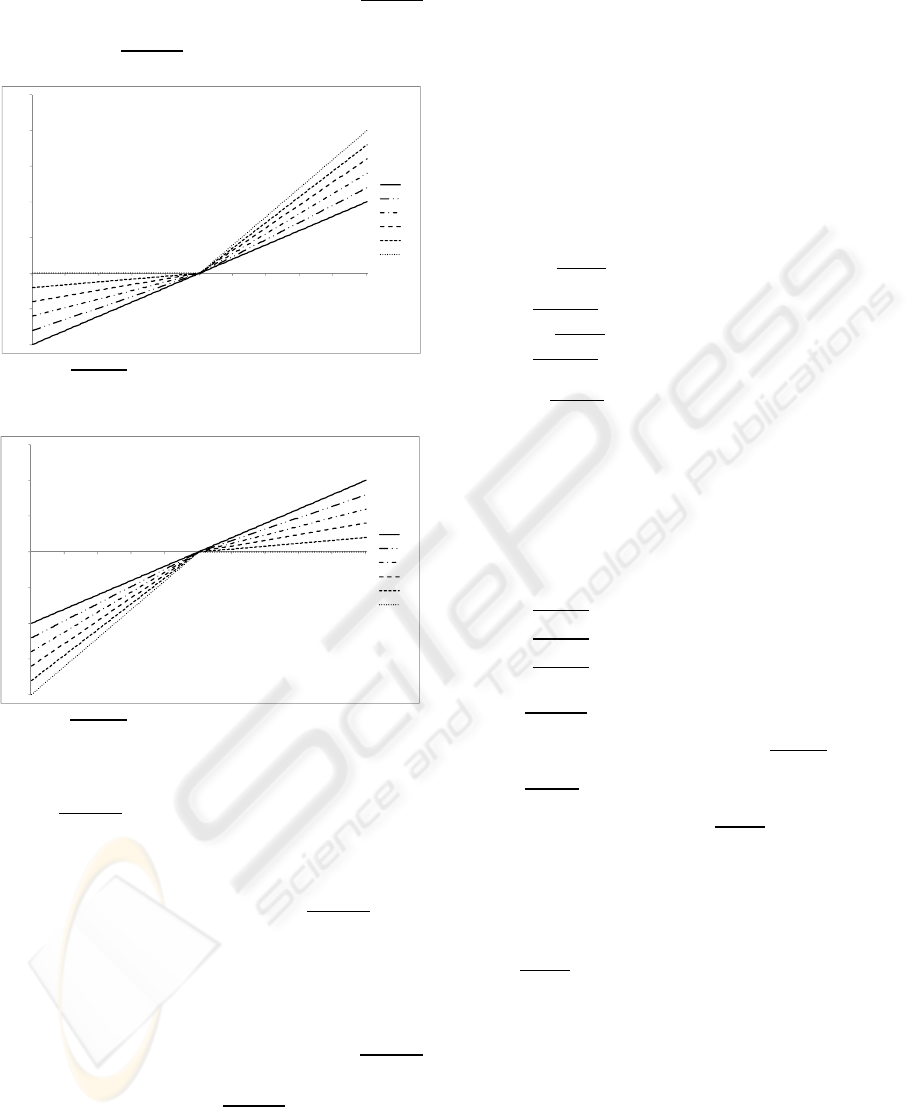
and less negative by increasing
, while never turn-
ing into a positive value (at most, when
,
gets equal to 0 for every
0). For example,
with
0.1,
is 10% higher than
.
Figure 1:
for agent
given
, for various
.
Figure 2:
for agent
given
, for various
In figure 2, a chart is shown with the various re-
sulting
, calculated according to equation 8,
for agent
, given
. This time, when compared to
the baseline result (
0), since
is the action
towards which the agent
has a negative bias, it’s
possible to notice that the resulting
is al-
ways lower (or equal, in case they are both 0) than
the original
calculated according to equation
6. In particular, higher
corresponds to more bias
(larger distance among the objective expected val-
ue), exactly opposite as it was before for action
.
Note that for a
1 (i.e.: maximum bias)
never gets past zero, so that
is performed if and
only if
- and hence
- is less than ze-
ro.
3.1 General Cases
The first general case (more than two possible ac-
tions and more than two categories of agents) is ac-
tually a strict super-case of the one formalized in
3.1. Each agent is endowed with an evaluation bi-
ased function derived from equations (7). Be
,
,…,
the set of agents, and
,
,…,
the set of possible actions to be
performed, then the specific agent
, with a posi-
tive bias for action
will feature such a biased
evaluation function:
:
|
|
…
|
|
|
|
|
|
…
|
|
(11)
This applies to each agent, of course by changing
the specific equation corresponding to her specific
positive bias. Even more general, an agent could
have a positive bias towards more than one action;
for example, if agent
has a positive bias for ac-
tions
and
and a negative bias for all the others,
the resulting equations will be:
:
|
|
|
|
|
|
…
|
|
(12)
In the most general case, for each EV
:
|
|
(13)
In case that two or more EV
a
have the same
value, the agent will perform the action towards
which it has a positive bias; in the case explored by
equation (12), in which the agent has the same posi-
tive bias towards more than one action, then the
choice among which action to perform, under the
same EV
a
, could be managed in various ways
(e.g.: randomly, stochastically and so on).
As a last general case, the agents could be a dif-
ferent positive/negative propensity towards different
actions. In this case, the variable to be used won’t
be the same for all the equations regarding an indi-
vidual agent. For example, given a set of
,
,…,
and a set of actions
,
,…,
, for each agent (
we have:
‐100
‐50
0
50
100
150
200
250
‐100 ‐80 ‐60 ‐40 ‐20 0 20406080100
0
0,2
0,4
0,6
0,8
1
‐200
‐150
‐100
‐50
0
50
100
150
‐100 ‐80 ‐60 ‐40 ‐20 0 20406080100
0
0,2
0,4
0,6
0,8
1
ICAART 2010 - 2nd International Conference on Agents and Artificial Intelligence
278

:
|
|
…
|
|
(14)
Besides being a fixed parameter, K could be a
stochastic value, e.g.: given a mean and a variance.
4 SIMULATED EXPERIMENTS
Some experiments were done in order to text the ba-
sic EBL equations introduced in paragraph 3.1. The
agents involved in the simulation can perform two
possible actions,
and
. The agents in the simu-
lation randomly meet at each turn (one to one) and
perform an action according to their EV. A payoff
matrix is used, in the form of:
Table 1: Example of payoff matrix.
Where
is the payoff originated when both
agents perform
,
is the payoff given to the
agents when one of them performs
and the other
one performs
and so on. Usually
and
are set
at the same value, for coherency. For each time-step
in the simulation, the number of agents performing
and
are sampled and represented on a graph.
Table 2: Payoff matrix for experiments 1 and 2.
1 -1
-1 2
The first baseline experiment reproduces the
classical RL equation (6), i.e.: with both
and
equals to zero. A total of 100 agents are used, with a
learning rate (
) set to 0.2. The payoff matrix used for
the experiment is shown in Table 2.
Action
is clearly
favored by the matrix, and coordination, in the form
of performing the same action, is rewarded, while
miscoordination punished.
In the first experiment, 50 agents start perform-
ing action
and 50 agents start performing action
. The results are depicted in figure 3; convergence
is subtle and stable, once the equilibrium is reached.
In the second experiment, a small bias towards
action
is introduced for fifty
agents (
= 0.1),
while the payoff matrix remains the same as in pre-
vious experiment. Agents
do not have a bias, but
all start playing action
; this will be different in
the following experiments, where unbiased agents
will start performing a random action. The results
are quite interesting, and depicted in figure 4.
Figure 3: Baseline experiment: no biased agents.
Figure 4: Experiment 1: biased Vs unbiased agents.
Even if action
is clearly favored by the payoff
matrix, after taking an initial lead in agents’ prefe-
rences, all the population moves towards action
.
This is due to the resilience of biased agents in
changing their mind; doing this way, the other 50
non-biased agents find more and more partners per-
forming action
, and thus, if they perform
they
get a negative payoff. In this way, in order to gain
something, since they are not biased, they are forced
to move towards the sub-optimal action
, preferred
by the biased agents. In order to give a social expla-
nation of this, we can think to the fact that often the
wiser persons adapt themselves to the more obstinate
ones, when they necessarily have to deal with them,
even if the outcome is not the optimal one, just not
to lose more. This is particular evident when the
wiser persons are the minority, or, as in our case, in
an equal number. At this point we wonder how
many “rotten apples” (i.e.: biased agents) are needed
to ruin the entire barrel (i.e.: turn away all the agents
from the optimal convergence), given the same
payoff matrix. With a series of ceteris paribus expe-
riments, we found the critical division to be 20/80;
the results are shown in figure 5. The unbiased
agents now start by performing a random action, in
0
20
40
60
80
100
12345678910111213141516171819
Actiona1 Actiona2
0
20
40
60
80
100
1 3 5 7 9 1113151719212325
Actiona1 Actiona2
LEARNING ACTION SELECTION STRATEGIES IN COMPLEX SOCIAL SYSTEMS
279

order to probe for the best move, and then adapt
themselves on the basis of their perceptions. On the
other hand, the biased agents start by performing
action
. In this way the agents performing
, both
biased and un-biased ones, when they meet an agent
performing
get a negative bias. Even if the op-
timal combination would be
, once again the
equilibrium is found on the suboptimal joint action,
which is
.
Figure 5: Experiment 2: Critical threshold.
Till now the advantage of performing join action
over
was evident (payoff 2 vs 1)
but not huge; in the next experiment, a new payoff
matrix is used, in the joint action
is re-
warded 3, instead of 2. The purpose is investigating
how much the previous threshold would increase
under these hypotheses. The empirical finding is
25/75, and the convergence is again extremely fast,
and much similar to the previous experiment. Even a
bigger advantage for the optimal action is soon nulli-
fied by the presence of just 25% biased agents, when
penalty for miscoordination exists. This explains
why sometimes suboptimal actions (or non-best
products) become the most spread and common. In
the real world, marketing could be able to bias a part
of the population, and a good distribution or other
politics for the suboptimal product/service could act
as a penalty for unbiased players when interacting
with biased ones. The following experiment investi-
gates the case with no penalty for miscoordination.
Table 3: Payoff matrix for experiments 3.
1 0
0 2
To explore the differences with experiment 1,
twenty biased agents were employed, out of 100.
The results are shown in figure 6.
Figure 6: Experiment 3: No penalty for miscoordination.
As it’s evident, now the results are less extreme,
in the sense that a part of the agents succeed in per-
forming the optimal action; though, many unbiased
agents are dragged along by the biased ones, to the
suboptimal action. Numerically speaking, about 50%
of unbiased agents become supporter of the subop-
timal action, even if the biased agents are a small
part of the population (20%).
This shows that penalty for miscoordination is
important, but not crucial, for averting the majority
of the population from the best possible choice.
5 FUTURE DEVELOPMENTS
While individual preferences are very important as a
bias factor for learning and action selection, when
dealing with social systems, in which many entities
operate at the same time and are usually connected
over a network, other factors should be kept into
consideration. In particular, the preferences of other
individuals with which a specific agent is in touch
can affect her choices, modifying the perception
mechanism described in equation 6. Once again, if
the goal is that of representing agents mimicking
human behaviour, then it’s not realistic to consider
perfect perception of the payoffs deriving from past
actions. Besides, Fragaszy and Visalberghi (2001)
agree that socially-biased learning is widespread in
the animal kingdom and important in behavioural
biology and evolution. It’s important to distinguish
between imitation and socially biased learning;
while the former is limited to de facto imitating the
behaviour of another individual (possible with some
minor changes), the second is referred to modifying
the possessed behaviour after the observation of oth-
ers’ behaviours. While imitation is most passive and
mechanical, social learning supposes a form of intel-
ligence in selecting how to modify the past behav-
iour, taking into account others’ experience.
0
20
40
60
80
100
1 3 5 7 9 11131517192123252729313335
Actiona1 Actiona2
0
20
40
60
80
100
1 3 5 7 9 1113151719212325
Actiona1 Actiona2
ICAART 2010 - 2nd International Conference on Agents and Artificial Intelligence
280

Box (1984) defines socially biased learning as: a
change in behaviour contingent upon a change in
cognitive state associated with experience that is
aided by exposure to the activities of social compan-
ions. The first part of this is already taken care by
RL methods (equation 6) and by the EBL proposed
in the previous sections. What is still lacking is the
bias coming from social companions, i.e.: other
agents coexisting in the same environment. In future
works a reputational based approach will be used, to
embed a form of social bias into the agents. This will
keep into consideration the payoffs deriving from
other agents’ actions, weighted by agents’ individual
reputations, acting as a bias for the equation defining
the RL strategy, along with EBL.
6 CONCLUSIONS
In this work a formal method for action selection is
introduced: it’s based on one step QL algorithm
(equation 6), but it takes into account individual
preference for one or more actions. This method is
designed to be used in simulation of social systems
employing MAS, where many entities interact in the
same environment and must take some actions at
each time-step. In particular, traditional methods do
not take into account human factor, in the form of
personal inclination towards different strategies, and
consider the agents as totally rational and able to
modify their behaviour based on an analytical payoff
function derived from the performed actions.
Ego biased learning is formally presented in the
most simple case, in which only two categories of
agents are involved, and only two actions are possi-
ble. That’s to show the basic equations and explore
the results, when varying the parameters.
After that, some general cases are faced and
equations are supplied, where an arbitrary number of
agents’ categories is taken into account, along with
an equally discretionary number of actions. There
can be many sub-cases for this situations, e.g.: one
action is preferred, and the others are disadvantaged,
or an agent has the same bias towards more actions,
or in the most general situation, each action can have
a positive or negative bias, for an agent.
Some simulations are run, and the results are
studied, showing how, even a small part of the popu-
lation, with a negligible bias towards a particular ac-
tion, can affect the convergence of a RL algorithm.
In particular, if miscoordination is punished, after
few steps all the agents converge on the suboptimal
action, which is the one preferred by the biased
agents. With no penalty for miscoordination, things
are less radical, but once again many non-biased
agents (even if not all of them) converge to the
suboptimal action. This shows how personal biases
are important in social systems, where agents must
coordinate or interact.
ACKNOWLEDGEMENTS
The authors wish to gratefully acknowledge as their
mentor prof. Gianpiero Bussolin, who applied new
technologies and simulation to Management and
Economics since 1964. This work is the ideal con-
tinuation of his theories.
REFERENCES
Box, H. O., 1984. Primate Behaviour and Social Ecology.
London: Chapman and Hall.
Chen M. K., 2008. Rationalization and Cognitive Disso-
nance: do Choices Affect or Reflect Preferences?
Cowles Foundation Discussion Paper No. 1669
Mataric M. J., 2004. Reward Functions for Accelerated
Learning. In Proceedings of the Eleventh International
Conference on Machine Learning.
Mataric, M. J., 1997. Reinforcement Learning in the
Multi-Robot domain. Autonomous Robots, 4(1)
Fudenberg, D., and Levine, D. K. 1998. The Theory of
Learning in Games. Cambridge, MA: MIT Press
Fragaszy, D. and Visalberghi, E., 2001. Recognizing a
swan: Socially-biased learning. Psychologia, 44, 82-
98.
Powers R. and Shoham Y., 2005. New criteria and a new
algorithm for learning in multi-agent systems. In Pro-
ceedings of NIPS.
Sharot T., De Martino B., Dolan R.J., 2009. How Choice
Reveals and Shapes Expected Hedonic Outcome. The
Journal of Neuroscience, 29(12):3760-3765
Sutton, R. S. and Barto A. G., 1998. Reinforcement Learn-
ing: An Introduction. MIT Press, Cambridge, MA. A
Bradford Book
Watkins, C. J. C. H. 1989. Learning from delayed rewards.
PhD thesis, Psychology Department, Univ. of Cam-
bridge.
LEARNING ACTION SELECTION STRATEGIES IN COMPLEX SOCIAL SYSTEMS
281
