SELF-ADAPTIVE MULTI-AGENT SYSTEM FOR

SELF-REGULATING REAL-TIME PROCESS

Preliminary Study in Bioprocess Control

Sylvain Videau, Carole Bernon and Pierre Glize

Institut de Recherche Informatique de Toulouse, Toulouse III University

118 Route de Narbonne, 31062 Toulouse, cedex 9, France

Keywords:

Adaptive control, Multi-agent systems, Cooperation, Bioprocess.

Abstract:

Bioprocesses are especially difﬁcult to model due to their complexity and the lack of knowledge available to

fully describe a microorganism and its behavior. Furthermore, controlling such complex systems means to

deal with their non-linearity and their time-varying aspects.

In order to overcome these difﬁculties, we propose a generic approach for the control of a bioprocess. This

approach relies on the use of an Adaptive Multi-Agent System (AMAS), acting as the controller of the bio-

process. This gives it genericity and adaptability, allowing its application to a wide range of problems and

a fast answer to dynamic modiﬁcations of the real system. The global control problem will be turned into a

sum of local problems. Interactions between local agents, which solve their own inverse problem and act in

a cooperative way, will enable the emergence of an adequate global function for solving the global problem

while fulﬁlling the user’s request.

An instantiation of this approach is then applied to an equation solving problem, and the related results are

presented and discussed.

1 INTRODUCTION

Regulating a dynamic system is a complex task, espe-

cially when we consider a real-world application im-

plying real-time constraints and limitations on com-

putational power. Biology offers some of the best ex-

amples of such systems when bioprocesses have to be

regulated.

Controlling a bioprocess is keeping a quasi-

optimal environment in order to allow the growth of

the expected microorganisms, while limiting and sup-

pressing any product with toxic characteristics. How-

ever, this task is difﬁcult, and this difﬁculty arises

from, on the one hand, the bioprocess complexity,

and, on the other hand, the amount of elements and

interactions between them that are to be taken into

account. Furthermore, controlling such a system im-

plies dealing with uncertainty coming from lags in

measures and delays in reactions.

Another point that has to be considered is the lack

of online (which means obtained directly from the

bioprocess) measures available. This limits the visi-

ble indicators of the consequences of the action of the

control, and leads the observer to rely on inferred data

in order to describe the biological state of the system.

In this paper, we present a generic approach

for controlling bioprocesses that uses an Adaptive

Multi-Agent System (AMAS). Section 2 presents an

overviewof the existing methodsof control before po-

sitioning our approach in section 3. This section also

expounds what are AMAS and details the features of

the agents composing the proposed one. Section 4

instantiates this system to an equation solving prob-

lem and gives some experimental results. Finally, the

conclusions and perspectives that this work offers are

discussed.

2 BIOPROCESS CONTROL: A

BRIEF OVERVIEW

Mathematically speaking, control theory is the sub-

ject of an extensive literature. Basically, two kinds

of control systems may be considered: the ﬁrst one

is an open loop, meaning that there is no direct con-

Videau S., Bernon C. and Glize P. (2010).

SELF-ADAPTIVE MULTI-AGENT SYSTEM FOR SELF-REGULATING REAL-TIME PROCESS - Preliminary Study in Bioprocess Control.

In Proceedings of the 2nd International Conference on Agents and Artiﬁcial Intelligence - Agents, pages 30-37

DOI: 10.5220/0002725100300037

 SciTePress

nection between the outputs of the controlled system

and its inputs. The control being carried out without

any feedback, it only depends on the model within

the controller itself. The second kind of control is a

closed loop, which is focused on the feedback, allow-

ing the control system to make actions on the inputs

by knowing the system’s outputs. In those two cases,

the function determiningthe control to apply is named

the control law. The control system presented here is

designed as a closed loop.

2.1 PID Control

Currently, the most widespread approach to control

bioprocesses is the Proportional-Integral-Derivative

(PID) controller. Controlling with such a tool means

that three different functions will be applied to the re-

ceived feedback, in order to select the adequate con-

trol. These functions are i) the proportional, which

computes the current error multiplied by a “propor-

tional constant”, ii) the integral, which takes into ac-

count the duration and magnitude of the error, by

summing their integral and multiplying by an “inte-

gral constant” and ﬁnally iii) the derivative, which es-

timates the rate of change of this error, allows to ob-

serve its variation, and multiplies it by a “derivative

constant”. These three functions are then summed.

However,several points need to be treated to make

this approach adaptive enough to follow the biopro-

cess dynamics; the different constants appearing in

the formulas have still to be deﬁned and a way to al-

low them to be adjusted during the bioprocess has to

be found. Such a modiﬁcation may be done by using

methods like Ziegler-Nichols (Ziegler and Nichols,

1942) or Cohen-Coon (Cohen and Coon, 1953).

This PID approach is quite generic, and can be ap-

plied to a wide range of control systems. However, its

performances in non-linear systems are inconsistent.

This drawback led to the hybridization of this method

by adding mechanisms relying on fuzzy logic (Visi-

oli, 2001), or artiﬁcial neural networks (Scott et al.,

1992).

2.2 Adaptive Control

The differences existing in the results coming from

distinct runs of the same bioprocess led us to study the

ﬁeld of adaptive control; these differences are for ex-

ample a noise addition or a delay in the chemical reac-

tions that modify the system dynamics. This problem

can be overcome by applying methods that dynami-

cally modify the control law of the controller.

There are mainly three different categories of

adaptive controller, the Model Identiﬁcation Adaptive

Control (MIAC), the Model Reference Adaptive Con-

trol (MRAC), and the Dual Control.

MIAC systems (Astrom and Wittenmark, 1994)

use model identiﬁcation mechanisms in order to en-

able the controller to create a model of the system

it controls. This model can be created from scratch

thanks to the observed data, or by using an already

known basis. The identiﬁcation mechanism updates

the model using values coming from inputs and out-

puts of the controlled system.

MRAC systems, suggested by (H.P. Whitaker and

Kezer, 1958), employ a closed loop approach modi-

fying the parameters of the controller thanks to one

or several reference models. This time, the system

does not create a model of the bioprocess, but it uses

an existing model to update the control law by ob-

serving the difference between the predicted output

and the measured ones. This adjustment is generally

applied by the use of the MIT rule (Kaufman et al.,

1994), which is a kind of gradient descent minimiz-

ing a performance criterion computed from the error

measured.

The last system is called Dual Controller (Feld-

baum, 1961) and is especially useful for controlling

an unknown system. In fact, such a control system

uses two kinds of actions, the ﬁrst one is a normal con-

trol, which aims at leading the system toward a certain

value, while the other one is a probing action, which

allows the controller to obtain more information on

the controlled system by observing its reaction. The

difference here is that the probing action is physically

applied on the system, and not only predicted by the

use of a model.

2.3 Intelligent Control

The last kind of controller is a subtype of the adap-

tive control, called intelligent control. It focuses on

the use of methods coming from artiﬁcial intelligence

to overcome problems linked to non-linearity and dy-

namic systems.

In the case of bioprocess control, the most used

intelligent controller is the artiﬁcial neural network

(ANN). Initially applied to bioprocesses to infer some

non-measurable variables, it was then used to control

such processes, or to improve already existing control

methods by providing adaptation. Furthermore, ANN

appear in pattern recognition control such as (Megan

and Cooper, 1992).

Unfortunately, the black box aspect of ANN is a

limit to their use in the bioprocess control. And even

if some works exist to reduce this aspect (Silva et al.,

2000), it is to the detriment of their adaptability.

Among the Artiﬁcial Intelligence techniques used

SELF-ADAPTIVE MULTI-AGENT SYSTEM FOR SELF-REGULATING REAL-TIME PROCESS - Preliminary Study

in Bioprocess Control

in intelligent control, we can also ﬁnd expert sys-

tems (Dunal et al., 2002) using knowledge databases

to select the control needed, and fuzzy logic (Visioli,

2001).

Bayesian controllers can be considered like in-

telligent controllers too, especially with the use of

Kalman ﬁlters. This mathematical approach uses two

distinct steps to estimate the state of the system. First,

a prediction step enables to estimate the current state

of the system using the estimation made in the previ-

ous state. Then, an update step improves this predic-

tion with the help of observationsmade on the system.

2.4 Limitations

However,these approaches generally lack of reusabil-

ity: the work required to apply them on a speciﬁc

bioprocess is useless for applying them on another

one. Indeed, the variables of mathematical models

are speciﬁcally chosen to ﬁt with a speciﬁc biopro-

cess, for example in the case of PID; and the learn-

ing set needed to train adaptive methods such as ANN

are quite difﬁcult to obtain on top of being meaning-

ful only in a restricted range of variations of the bio-

process. This over-speciﬁcation limits the predictive

power of the controller when the bioprocess diverges

from the expected scheme, and so, such a controller

is unable to bring back the bioprocess into a desired

state. Generally, black box models are poor at ex-

trapolating and weak in accomodating lags (Alford,

2006). The approach presented in this work, and its

perspectives,aim at reducing the impact of such draw-

backs, by offering a generic and adaptive control us-

ing a Multi-Agent System (MAS).

3 CONTROL MULTI-AGENT

SYSTEM (CMAS)

Using a MAS to control and manage a process is

an approach already experimented, for example in

(Taylor and Sayda, 2008). However, the complexity

brought by a bioprocess implies the use of an adap-

tive architecture to organize the CMAS. As a result,

the principles governing the MAS proposed for con-

trolling a system in real-time come from the Adaptive

Multi-Agent System (AMAS) theory (Gleizes et al.,

1999). This AMAS has to determine which control

to apply on the bioprocess in order to drive the val-

ues of certain variables to reach a user-deﬁned ob-

jective. This section begins by a description of these

AMAS principles before giving an overview of the

MAS and its positioning in the global control mech-

anism. The abilities and behavior of the agents com-

posing this AMAS are then detailed before delineat-

ing the generic aspects of the proposed approach in

order to instantiate it according to a speciﬁc problem.

3.1 The AMAS Approach

The functional adequacy theorem (Gleizes et al.,

1999) ensures that the global function performed by

any kind of system is the expected one if all its parts

interact in a cooperative way. MAS are a recog-

nized paradigm to deal with complex problems and

the AMAS approach is focused on the cooperative be-

havior of the agents composing a MAS.

Here, cooperation is not only a mere resource or

task sharing, but truly a behavioral guideline. This

cooperation is considered in a proscriptive way, im-

plying that agents have to avoid or solve any Non Co-

operative Situation (or NCS) encountered. Therefore,

an agent is considered as being cooperative if it veri-

ﬁes the following meta-rules:

• c

per

: perceived signals are understood without

ambiguity.

• c

dec

: received information is useful for the

agent’s reasoning.

• c

act

: reasoning leads to useful actions toward

other agents.

When an agent detects a NCS ( ¬c

per

∨ ¬c

dec

∨

¬c

act

), it has to act to come back to a cooperative

state. One of the possible actions such an agent may

take is to change its relationships with other ones

(e.g., it does not understand signals coming from an

agent and stops having relationships with it or make

new ones for trying to ﬁnd other agents for helping it)

and therefore makes the structure of the global sys-

tem self-organize. This self-organization led by co-

operation changes the global function performed by

the system that emerges from the interactions between

agents. The MAS is thus able to react to changes

coming from the environment and therefore becomes

adaptive.

3.2 Structure of the CMAS

The AMAS described in this paper relies on the use of

an existing model of the bioprocess it has to control.

This model may be composed of any kind of different

submodels (mathematical equations, ANN, MAS...)

because this point only inﬂuences the instantiation of

our agent detailed in section 3.2.2. Basically, a super-

position of agent composing the CMAS on the bio-

process model must be done in order to create the

structure of the CMAS. Figure 1 illustrates an exam-

ple of such a superposition where one agent is associ-

ICAART 2010 - 2nd International Conference on Agents and Artificial Intelligence

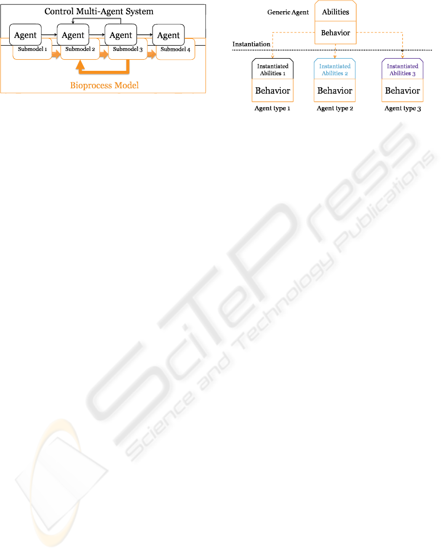
Figure 1: Example of superposition of agents on the biopro-

cess model.

ated with one submodel, but it would also be possible

to describe one submodel with several agents. This

choice is up to the system designer and offers an im-

portant ﬂexibility, especially in the granularity of the

created system.

When the general design of the CMAS is ob-

tained, the description of the agents that are compos-

ing it is performed following the AMAS approach.

3.2.1 Generalities on CMAS Agents

Each of the agents composing the CMAS represents

a variable, or a set of variables such as the quanti-

ties of different elements in a bioprocess, on which

they have objectives of different criticity. This critic-

ity symbolizes the priority of the objective, and agents

can compute it thanks to the difference between their

current value and the expected one. The main goal of

an agent is to satisfy its most critical objective, which

means to bring a variable toward a certain value.

Agents that compose the CMAS follow a common

model, but they can be instantiated in different ways.

This phenomenon is detailed in Figure 2, underlin-

ing the fact that even if their ability are implemented

differently, their behavior stay the same and so, the

MAS is always composed of cooperative agents that

are able to interact with one another.

3.2.2 Abilities of CMAS Agents

As stated by the AMAS approach, an agent has a

strictly local view. From this local point of view, it

computes its own objective which may be modiﬁed

by the communication between agents. As a result,

an agent must be able to evaluate the current objec-

tive that it has to achieve, and to update it according to

the evolution of its criticity. This ability includes the

need to communicate with other agents, and to man-

age a set of received messages, by sorting them, or

aggregating them according to the problem, in order

to extract the current objective, which has the highest

criticity.

Figure 2: Instantiation of agents.

Our control system supposes the existence of a

model of the bioprocess which has to be controlled.

This model is used by the agents, which are able to

extract certain abilities from it.

These abilities are the observation and the use of

a local part of the bioprocess model. An agent is able

to virtually inject some values (without any real con-

trol action) at the input points of the local model it

observes in order to extract the corresponding output

values. These observations enable this agent to have

an idea of the variation direction that it has to apply in

input for obtaining a desired output. Therefore, this

mechanism grants an agent the abilities of its own di-

rect problem solving, and gives it the tools needed to

treat its own inverse problem, by determining which

inputs it has to apply for achieving a certain output.

For example, let us consider an equation y = f(x).

At time t, this equation is y

= f(x

Then, at t

′

= t + 1, we obtain y

′

= f(x

+ ∆x), this

∆x being a light variation of x.

Finally, by observing the sign of y

′

− y

, the agent

is able to ﬁnd the modiﬁcation ∆x which moves y

closer to its objective.

Thus, agents are able to deal with their inverse

problem without needing a model that describes their

inverse problem, such as the lagrangian.

Finally, each agent is able to compute its own ob-

jective, which is a set of values that the agent aims

at. This computation depends on the communication

between agents (described in part 3.2.3), and on the

observation that an agent is making on its own local

model. This objective can also be established by the

user.

3.2.3 Behavior of CMAS Agents

The main mechanism guiding the behavior of the

agents rests on a model in which this behavior is di-

vided into two categories: the Nominal and the Co-

operative one. The Nominal behavior describes the

default behavior of an agent, the one used when this

SELF-ADAPTIVE MULTI-AGENT SYSTEM FOR SELF-REGULATING REAL-TIME PROCESS - Preliminary Study

in Bioprocess Control

agent has no need to process one of the Non Co-

operative Situations (NCS) described in 3.1, while

the Cooperative behavior enables it to overcome the

NCS met during the control. This Cooperative be-

havior is itself divided into three different behaviors.

First, Tuning consists in trying to tweak parameters to

avoid or solve a NCS. If this behavior fails to make

an agent escape from this NCS, Reorganization takes

place. This Reorganization aims at reconsidering the

links established with other agents. Finally, Evolution

enables the possibility for an agent to create another

agent, or to self-destruct because it thinks itself as to-

tally useless.

In the bioprocess control, the Nominal behavior

has been instantiated in the following way. The agents

communicate with one another in order to share their

non-satisfaction degrees, and solve them if possi-

ble. This non-satisfaction degree is tied to a vari-

able which value does not satisfy the objectives of the

agent. Two different kinds of messages can be sent:

• A Request message which expresses a non-

satisfaction of the sending agent and asks for an

action of control in order to change the value of

the problematic value.

• An Answer message which notiﬁes an applied

control, or the observation of the modiﬁcation of

a value observed from the model by the agent.

As a consequence, even if two agents come from

different instantiations, they share the same Nominal

behavior which consists in sending requests asking

for the modiﬁcation of values that did not satisfy the

agent, and acting if possible in order to answer those

requests by carrying out a control action.

These two points are completed by the Coopera-

tive behavior of Tuning stating that an agent receiving

a request, to which it cannot answer positively, is able

to modify it for conveying this modiﬁcation towards

the other agents linked with it. This modiﬁcation is

applied in order to make the request relevant to the re-

ceiving agent. It ensures that this request will be use-

ful and comprehensible for these agents, by asking for

modiﬁcations on variables that they know about. The

inverse problem solving ability of an agent is used

during this modiﬁcation to decide which are the ad-

justments needed on the inputs to obtain the desired

output.

The control can also be partially done when an

agent is unable to make it completely; for example,

if the agent is not permitted to make a modiﬁcation of

sufﬁcient amplitude. In this case, it makes the max-

imum control possible and then, sends an answer to

notify this modiﬁcation to the other agents. Thus, if

this objective is still the most critical for the agent

source of the request, then a request related to the

same objective will be sent again, and will ﬁnally be

answered positively when another control will be pos-

sible. So, this behavior is still a Tuning behavior.

Eventually, in order to solve a speciﬁc control

problem with this approach, our agents’ abilities have

to be instantiated according to the problem. For exam-

ple, the methods used to observe and use models on

which the agents are created must be deﬁned depend-

ing on the kind of model used. The way the agents

compute their current objective has also to be instan-

tiated. To summarize, all the abilities described in

section 3.2.2 may be implemented in different ways,

without modifying the behavior of the agents. So, the

MAS created for the control of bioprocesses can be

composed of any number of different kinds of agents,

provided that these agents possess the described abil-

ities, instantiated to fulﬁll their role, and follow the

same behavior.

In order to evaluate the control system that was de-

veloped, an instantiation to an equation solving prob-

lem was carried out.

4 EXAMPLE OF AN EQUATION

SYSTEM

The goal of this example is to modify dynamically the

values of some variables to fulﬁll some objectivesthat

the user put on other variables. These objectives are

threshold values that the variable must reach and the

user can modify them during the simulation.

4.1 Description of Agents

Two different types of agents were instantiated:

Equation Agents and Variable Agents.

Figure 3 explains how the MAS is generated from

a mathematical equation. First, a Variable Agent is

created for each variable appearing in the different

equations. A Variable Agent is an agent that can make

a control action by modifying the value of the math-

ematical variable associated with it. The model used

by this agent is simply a model of the mathematical

variable, namely the variable itself. Therefore, in-

verse and direct problem solvings are trivial for such

an agent, the result being the value of the mathemat-

ical variable. Finally, a Variable Agent can be the

target of user-deﬁned objectives deﬁning a value to

achieve.

After Variable Agents are created, an Equation

Agent is added for each mathematical equation be-

longing to the system to solve. Each Equation Agent

relies on the model of the mathematical equation it

ICAART 2010 - 2nd International Conference on Agents and Artificial Intelligence

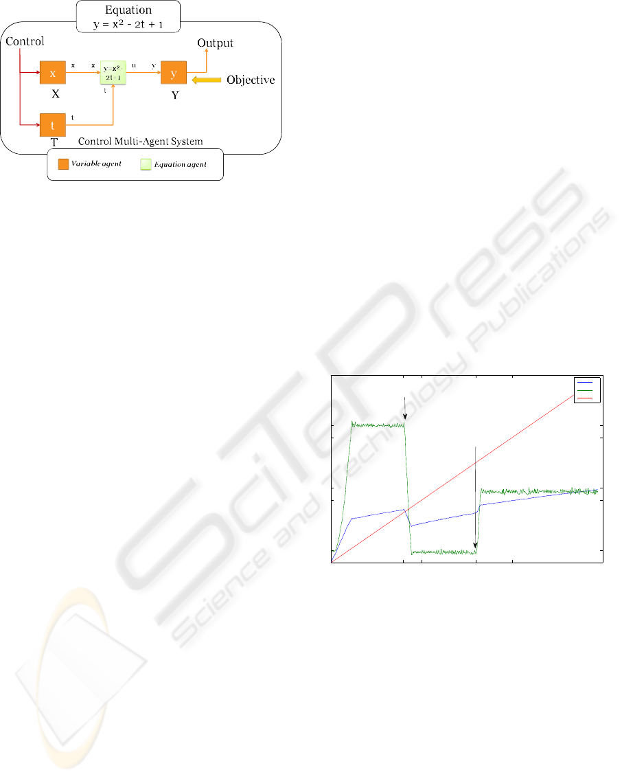
Figure 3: Creation of the CMAS from an equation.

represents and this agent is able to know any output

generated from a set of inputs thanks to its direct prob-

lem solving ability. Here, the inverse problem solving

mechanism uses the same model, an Equation Agent

tunes the inputs and, by observing the generated out-

puts, is able to estimate the modiﬁcation needed to get

closer to its objectives. However, while an Equation

Agent is able to compute the amount and the direction

of the modiﬁcation to apply, it cannot make any con-

trol action. It has then to create requests and sends

them to the corresponding Variable Agents.

When this step is done, an objective is allocated

to a Variable Agent representing the output of the sys-

tem, e.g., the agent Y on Figure 3. Agents X and T

are able to apply control actions.

Finally, a last type of agent, named Independent

Variable Agents, is derived from the Variable Agent

one to which it adds a speciﬁc ability. Such an agent

cannot make control actions but, instead, it represents

a variable which value is modiﬁed over time, accord-

ing to an inner function. That means that an Inde-

pendent Variable Agent may receive requests but will

never be able to fulﬁll them. On the other hand, at

each simulation step, it will send an answer to no-

tify the modiﬁcation of its variable to other agents.

The interest of this agent is to underline how the other

Variable Agents act to make up for the drift brought

by this uncontrolled modiﬁcation.

The relationships between the agents composing

the equation control system are as follows: an Equa-

tion Agent is linked, at its inputs, with every Variable

Agent or Independent Variable Agent from the math-

ematical equation. Its outputs are connected with the

Variable Agent representing the result variable. Com-

munication between agents follows these links.

4.2 Experimental Results

This section describes three examples of equation sys-

tems, highlighting different aspects of the presented

approach. In these examples, the agents are con-

strained to update their value progressively, meaning

that Equation Agents do not send the correct value

that they have to reach to Variable Agents, but rather

a modiﬁcation step toward this value. This fact comes

from the implementation of the inverse problem solv-

ing on Equation Agents, whose goal is to drive its in-

puts gradually toward the expected value, and not in

a single jump. On top of that, when a Variable agent

is created, it is named after the capital letter of the

mathematical variable that it represents.

4.2.1 Controlling Single Polynomial Equation

This example consists of a single equation y = x

−

2t + 1, made up of a Variable Agent Y, which re-

ceives objectives from the user. Inputs are a Variable

Agent X and an Independent Variable Agent T. Dur-

ing the process, the objective of agent Y is changed

two times, depicted by arrows on Figure 4. Initially,

its goal is 11, then the two changes occur at time 400

and time 800 when the objective is respectively set to

1 and 6.

0 500 1000 1500400 800

Simulation Step

Value

Objective change 1

y = 1

Objective change 2

y = 6

Figure 4: Results from the control of an introductory exam-

ple.

Results presented in Figure 4 (on which time is

expressed as simulation steps) highlight the reaction

of the control performed by X, which compensates

the uncontrolled evolution of T, while reacting to the

objectives changes made on Y. The delay to reach the

objective value when Y changes its goal comes from

a maximum limit on the modiﬁcation enforceable for

each simulation step.

4.2.2 Controlling Multiple Polynomial

Equations

This example, presented in Figure 5, is composed

of 4 different equations, with a total of 10 variables

SELF-ADAPTIVE MULTI-AGENT SYSTEM FOR SELF-REGULATING REAL-TIME PROCESS - Preliminary Study

in Bioprocess Control

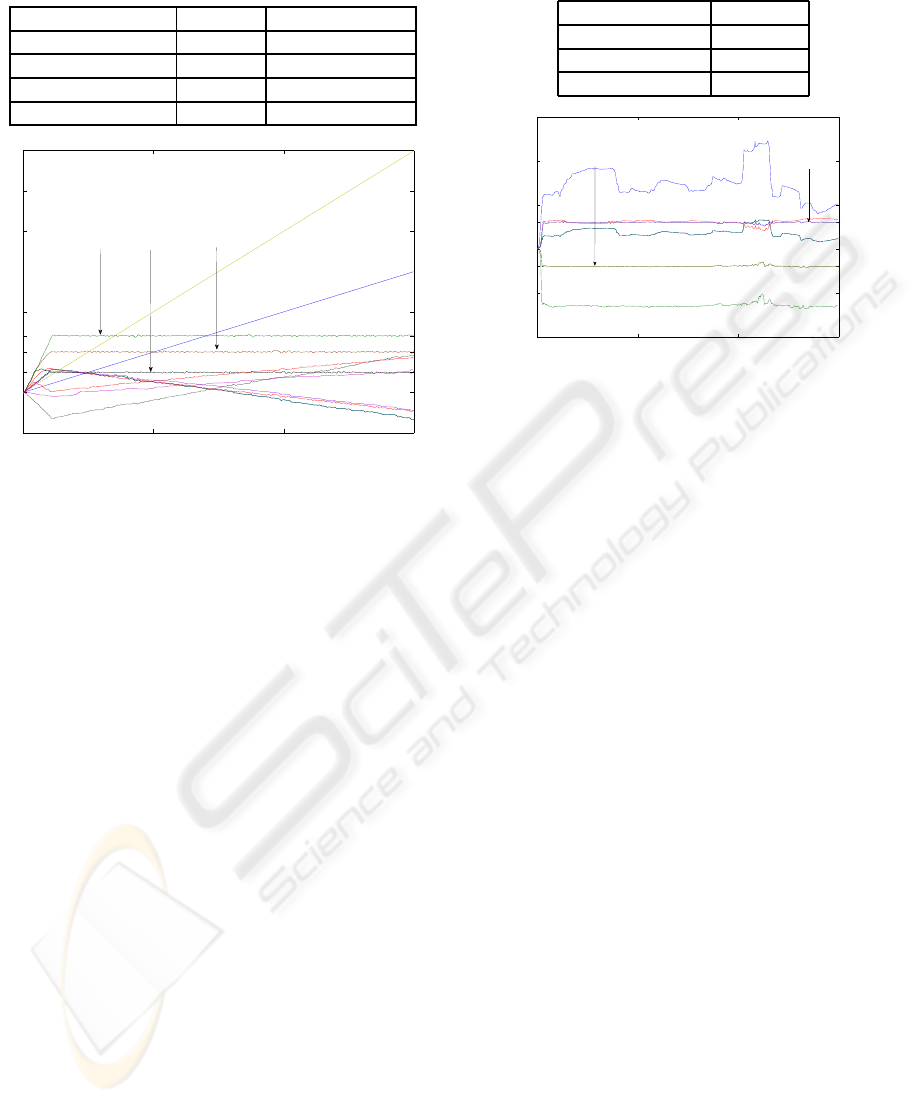
Table 1: “Multiple Polynomial” Equation Data.

Equations Variables Independent Var.

u = 0.2x+ y+ 0.3t u, x, y t

v = 0.8y + z v, y, z

w = 0.4x− a+ o w, x, a o

x = d − 0.4e x, d, e

0 500 1000 1500

−10

Simulation Step

Value

W = 14

V = 5

U = 10

Figure 5: Results from the control of the multiple polyno-

mial example.

whereof two of them are independent. Three objec-

tives are deﬁned at time 0 (10 for U, 5 for V and 14

for W) and remain static during the process. Those

three variables are selected to receive objectives be-

cause they represent the outputs of the system, they

are not used as an input for another equation. The full

equations data are detailed in Table 1.

This example shows how multiple equations, that

share variables, and can send antagonist objectives to

them, are able to fulﬁll all the deﬁned objectives. The

values of the variables that are undergoing the greater

changes are those of the non-shared variable. On top

of that, the noise coming from the Independent Vari-

able Agents is reduced thanks to the controls done by

the Variable Agents.

Another interesting point comes from the adaptive

feature of such a system. Indeed, several simulations

were run to solve the presented problems, and we can

observe that, given the few constraints on some vari-

ables, the system is able to ﬁnd different balanced

states. During each time step, all the agents compos-

ing the CMAS can act, but due to the stochastic or-

der on which they behave, some delays may appear in

the messages transmission. Therefore, some modiﬁ-

cations occur before some others, implying a different

dynamics. In those different cases, the CMAS is able

to converge toward a stable state respecting the con-

straints. This fact can model a kind of management

of noise coming from time delays, and highlights the

Table 2: “Interdependent” Equation Data.

Equations Variables

u = 0.3x+ 0.8y u, x, y

v = 0.2u + 0.4z v, u, z

x = 0.2v+ 0.3m x, v, m

0 500 1000 1500

−10

−5

−2

Simulation Step

Value

V = −2

U = 3

Figure 6: Results from the control of the interdependent

equations example.

robustness of the presented approach.

4.2.3 Controlling Interdependent Equations

The last example deals with the loops that appear in

the controlled system, a common phenomenon in the

equations used to describe bioprocesses. The results

available on Figure 6 are made up of 3 equations, de-

tailed in the Table 2, and possess 2 static objectives.

The Variable agent V has to reach the value −2 while

the Variable agent U aims toward 3.

This example underlines the message manage-

ment ability of the Variable Agents. Indeed, an agent

has to determine if a received request is still relevant.

Here, we can have requests that are making a full loop

and so, the agents must take this into account to avoid

a divergence of results, by summing unnecessary re-

quests.

Finally, it is noticeable that those three aspects,

which are the dynamic change of objectives, indepen-

dent variables and loops, presented here on separate

examples, are managed in the same way when they

are combined on the same equation system.

5 CONCLUSIONS &

PERSPECTIVES

This paper focuses on the control of real-time, dy-

namic and non-linear problems, and presents a ﬁrst

step towards an adaptive control of bioprocesses. The

approach given uses an AMAS made up of different

types of generic cooperativeagents. The behavior and

ICAART 2010 - 2nd International Conference on Agents and Artificial Intelligence

abilities of these agents, as well as their relationships,

were detailed. An instantiation of this generic ap-

proach was applied to an equation solving problem

in order to prove the feasibility of this kind of control

on different kinds of equations. The results obtained

highlight the relevance of this approach, and its adapt-

ability to a wide range of problems, especially the

bioprocess control, a bioprocess being often modeled

thanks to equations systems.

Currently, the application of the proposed ap-

proach to a full bioprocess model, with a true bio-

logical meaning, modeling the bioreactor physics and

the evolution of microorganisms, is under develop-

ment. This application will enable evaluating the per-

formances of our control system, while validating its

scalability, such a model being composed of hundred

of equations.

On top of that, we are considering the time as-

pects, especially lags and delays coming from the

scale diversity on which reactions occur. The design

of a mechanism to manage those delays is in progress

with a twofold aim. The ﬁrst one is to measure the im-

pact of different kinds of time constraints on the con-

vergence of the system towards its objectives and the

second one is to improvethe robustness of this system

while applied to strongly non-linear problems.

The ﬁnal objective of this work is to combine this

control system with another AMAS which dynami-

cally models the bioprocess. Thus, the model needed

by the agents belonging to the control system will it-

self be composed of agents, reducing the work of in-

stantiation of the control agents. Therefore, the global

control system will be viewed as a Model Identiﬁca-

tion Adaptive Control.

REFERENCES

Alford, J. S. (2006). Bioprocess control: Advances and

challenges. Computers & Chemical Engineering,

30:1464–1475.

Astrom, K. J. and Wittenmark, B. (1994). Adaptive Control.

Addison-Wesley Longman Publishing, Boston, MA,

USA.

Cohen, G. H. and Coon, G. A. (1953). Theoretical consider-

ation of retarded control. Journal of Dynamic Systems,

Measurement, and Control, pages 827–834.

Dunal, A., Rodriguez, J., Carrasco, E., Roca, E., and Lema,

J. (2002). Expert system for the on-line diagnosis of

anaerobic wastewater treatment plants. Water science

and technology, 45:195–200.

Feldbaum, A. (1960-1961). Dual control theory i-iv.

Automation Remote Control, 21,22:874–880, 1033–

1039, 1–12, 109–121.

Gleizes, M.-P., Camps, V., and Glize, P. (1999). A The-

ory of Emergent Computation based on Cooperative

Self-organization for Adaptive Artiﬁcial Systems. In

4th European Congress of Systems Science , Valencia

Spain.

H.P. Whitaker, J. Y. and Kezer, A. (1958). Design of model

reference adaptive control systems for aircraft. Tech-

nical Report R-164, MIT.

Kaufman, H., Bar-Kana, I., and Sobel, K. (1994). Direct

adaptive control algorithms: theory and applications.

Springer-Verlag, NY, USA.

Megan, L. and Cooper, D. J. (1992). Neural network

based adaptive control via temporal pattern recogni-

tion. The Canadian Journal of Chemical Engineering,

70:1208–1219.

Scott, G. M., Shavlik, J. W., and Ray, W. H. (1992). Re-

ﬁning pid controllers using neural networks. Neural

Computation, 4(5):746–757.

Silva, R., Cruz, A., Hokka, C., and Giordano, R. (2000).

A hybrid feedforward neural network model for the

cephalosporin c production process. Brazilian Journal

of Chemical Engineering, 17:587–597.

Taylor, J. H. and Sayda, A. F. (2008). Prototype design

of a multi-agent system for integrated control and as-

set management of petroleum production facilities.

In Proc. American Control Conference, pages 4350–

4357.

Visioli, A. (2001). Tuning of pid controllers with fuzzy

logic. IEE Proceedings - Control Theory and Appli-

cations, 148(1):1–8.

Ziegler, J. G. and Nichols, N. B. (1942). Optimum settings

for automatic controllers. Transaction of the ASME,

64:759–768.

SELF-ADAPTIVE MULTI-AGENT SYSTEM FOR SELF-REGULATING REAL-TIME PROCESS - Preliminary Study

in Bioprocess Control