FREE SPACE COMPUTATION FROM STOCHASTIC OCCUPANCY

GRIDS BASED ON ICONIC KALMAN FILTERED DISPARITY MAPS

Carsten Høilund, Thomas B. Moeslund, Claus B. Madsen

Laboratory of Computer Vision and Media Technology, Aalborg University, Denmark

Mohan M. Trivedi

Computer Vision and Robotics Research Laboratory, University of California, San Diego, U.S.A.

Keywords:

Free space, Stereo vision, Kalman ﬁltering, Stochastic occupancy grid.

Abstract:

This paper presents a method for determining the free space in a scene as viewed by a vehicle-mounted camera.

Using disparity maps from a stereo camera and known camera motion, the disparity maps are ﬁrst ﬁltered by

an iconic Kalman ﬁlter, operating on each pixel individually, thereby reducing variance and increasing the

density of the ﬁltered disparity map. Then, a stochastic occupancy grid is calculated from the ﬁltered disparity

map, providing a top-down view of the scene where the uncertainty of disparity measurements are taken into

account. These occupancy grids are segmented to indicate a maximum depth free of obstacles, enabling the

marking of free space in the accompanying intensity image. The test shows successful marking of free space

in the evaluated scenarios in addition to signiﬁcant improvement in disparity map quality.

1 INTRODUCTION

Autonomous robots in homes and factories are be-

coming ever more prevalent. These robots perform

automatic analysis of their surroundings to determine

their position and where they can move, and ideally to

determine what their surroundings consist of and who

might be present. This makes it natural to include

cameras for functions such as object recognition, face

recognition, and so forth.

To reduce the number of components on board, it

would be beneﬁcial to use the image data for naviga-

tion as well. One important aspect of navigation is

free space. This needs to be established on-the-ﬂy for

the robot to be able to handle dynamic environments,

such as doors opening or outdoor environments. De-

termining the depth of a scene is difﬁcult based on 2D

images, but easier with 3D data, leading to a choice of

stereo images. It is important to have accurate depth

information to reliably determine the free space.

The focus of this paper is to improve the 3D data

used for determining free space, obtainable from e.g.

monocular camera (Li et al., 2008), stereo camera

(Murray and Little, 2000), and omni-directional cam-

eras (Trivedi et al., 2007).

1.1 This Work

In this work we will use stereo cameras to simultane-

ously provide images and depth. We will not assume

forward pointing cameras, as seen in e.g. (Badino

et al., 2007), but rather allow for arbitrary camera

poses. The stereo images and initial depth estima-

tion are provided by a TYZX stereo camera with a

22 cm baseline (TYZX, 2009). The depth estima-

tion is reﬁned by applying ego-motion to a previous

frame thereby transforming it to correspond to the

new viewpoint, and subsequently merging the trans-

formed frame and the current frame, creating a more

accurate estimation. The reﬁned depth estimation is

used to determine the free space around the camera.

2 DEPTH ESTIMATION

Disparity is the measure of difference in position of a

feature in one image compared to another image.

This can be used to infer the depth of the feature. Sev-

eral methods of estimating disparity exist and the cru-

cial point in this work is to have an accurate measure-

ment to reliably determine free space. Knowledge of

the noise in the estimation process can signiﬁcantly

164

Høilund C., B. Moeslund T., B. Madsen C. and M. Trivedi M. (2010).

FREE SPACE COMPUTATION FROM STOCHASTIC OCCUPANCY GRIDS BASED ON ICONIC KALMAN FILTERED DISPARITY MAPS.

In Proceedings of the International Conference on Computer Vision Theory and Applications, pages 164-167

DOI: 10.5220/0002830601640167

 SciTePress

improve the system. In our case the distribution of

noise has been found to be Gaussian in image space

and hence the Kalman ﬁlter (Kalman, 1960) can be

applied.

2.1 Iconic Kalman Filter

The Kalman ﬁlter is a recursive estimation method

that efﬁciently estimates and predicts the state of a

discretized, dynamic system from a set of potentially

noisy measurements such that the mean square error

is minimized, giving rise to a statistically optimal es-

timation. Only the previous measurement and the cur-

rent measurement are needed.

The general Kalman ﬁlter equations are not di-

rectly applicable to a stream of images without some

additional considerations. If an N × M disparity map

was treated as a single input to one Kalman ﬁlter

the measurement covariance matrix R would consist

of (N × M)

values, which quickly becomes a pro-

hibitively large number. To make an implementation

feasible, each pixel is assumed independent and con-

sequently assigned a separate Kalman ﬁlter. A pixel-

wise Kalman ﬁlter is said to be iconic (Matthies et al.,

1989).

The ﬁlter is applied to disparities, meaning it is

the disparity value that is estimated. The pixel coordi-

nates are still used when applying the motion model,

but not Kalman ﬁltered. The state vector is therefore

just a scalar, i.e. x

= x

= d

2.1.1 State, Measurement and Motion Models

The measurement is the disparity value supplied by

the stereo camera. When the camera moves, the pre-

vious disparity map will in general not represent the

new camera viewpoint. Since depth is available for

each pixel they can be moved individually accord-

ing to how the camera was moved, effectively pre-

dicting the scene based on the previous disparity map

and the ego-motion information of the camera yield-

ing two disparity maps depicting the same scene from

the same view point; a prediction and a measurement.

The ego-motion in this context is linear in world

space but since image formation is non-linear,the mo-

tion becomes non-linear in image space. The standard

Kalman ﬁlter assumes a linear system which means

it cannot handle the application of ego-motion when

working in image space. Therefore, the state predic-

tion is handled outside of the Kalman ﬁlter by tri-

angulating the input into world space, applying ego-

motion as X

= M

t−1

+ M

(where M

is transla-

tion and M

is rotation), and then back-projecting the

result into image space. The Kalman ﬁlter therefore

only handles the state variance.

Support for arbitrary camera poses is accom-

plished by including a transformation of the ego-

motion information to the coordinate system of the

camera, given as ω

and ω

for translation and rota-

tion, respectively.

The complete motion model will be referred to as

the function Φ(.):

t|t−1

= Φ(x

t−1|t−1

, M

, ω

) (1)

2.1.2 Noise Models

The process and measurement variance are both

scalars and assumed to be constant, i.e. Q = q

and

R = r

. The process variance q

reﬂects the conﬁ-

dence in the predictions and is set to a small number

to ﬁlter out moving objects (e.g. 0.001). The mea-

surement variance r

represents the noise in the dis-

parity values and is determined by measuring the pre-

cision of the stereo camera. The Kalman gain K is ef-

fectively a weighting between the prediction and the

measurement based on the relative values of q

and

The state variance P is also a scalar, hence P = p.

It is initially set to r

, and from there on maintained

by the Kalman ﬁlter.

2.1.3 Predict Phase and Update Phase

The ﬁnished iconic Kalman ﬁlter equations become:

Predict

t|t−1

= Φ(x

t−1|t−1

, M

, ω

) (2)

t|t−1

= P

t−1|t−1

+ q

(3)

Update

= P

t|t−1



t|t−1

+ r



−1

(4)

t|t

= x

t|t−1

+ K



− x

t|t−1



(5)

t|t

= (1− K

t|t−1

(6)

where x is the estimated state, Φ(.) is the mo-

tion model, M

is the ego-motion as trans-

lation/rotation matrices, ω

/ω

is the transla-

tion/rotation of ego-motion to camera coordinate sys-

tem, P is the state variance, q

is the process variance,

y is the measurement variable, K is the Kalman gain,

and r

is the measurement variance.

2.1.4 Update Phase Merging

After the prediction phase has completed and a new

disparity map has been calculated, the update phase

begins. For each pixel, one of three scenarios occur:

FREE SPACE COMPUTATION FROM STOCHASTIC OCCUPANCY GRIDS BASED ON ICONIC KALMAN

FILTERED DISPARITY MAPS

165

1) No measurement exists for the position of the

predicted pixel. The disparity present is simply kept

as-is. A disparity is only carried over a certain num-

ber of consecutive frames before being discarded to

prevent stale pixels from degrading the result.

2) No predictions exists for the position of the

measured pixel, and the disparity is kept as-is.

3) Both exist. To ﬁlter out noise, a measurement

is checked against the prediction it is set to be merged

with by applying the Mahalanobis 3-sigma test (Ma-

halanobis, 1936). If a measurement is within three

standard deviations (three times the square root of r

)

of the mean (the prediction)in a given Gaussian distri-

bution, it is merged with the prediction by the Kalman

ﬁlter. If it fails, it replaces the prediction only if the

prediction is young (to prevent spurious pixels from

keeping correct measurements out) or deemed stale

(to ﬁlter out pixels that have drifted).

3 FREE SPACE ESTIMATION

3.1 Stochastic Occupancy Grid

With a disparity map (and consequently a reconstruc-

tion of the world points), the free space where a ve-

hicle can navigate without collision can be computed

by way of an occupancy grid (Elfes, 1989). An oc-

cupancy grid can be thought of as a top-down view

of the scene, with lateral position along the horizontal

axis and depth along the vertical axis. In a stochas-

tic occupancy grid (Badino et al., 2007) the intensity

of each cell denotes the likelihood that a world point

is at the lateral position and depth represented by the

cell. A world point can therefore occupy more than

one cell. How large an area the world point affects

depends on the variance (noise) associated with the

point. There exists various occupancy grid represen-

tations. In this paper, the polar occupancy grid is cho-

sen.

3.2 Free Space

Free space is determined with a combination of the

occupancy grid and the underlying disparity map.

3.2.1 Occupancy Grid Segmentation

Each cell in an occupancy grid contains a value rep-

resenting the probability of that cell being occupied.

The grid is segmented by traversing it from near to far,

stopping when the value of a cell exceeds a threshold.

The depth of that cell is the maximum depth likely to

be free of obstacles.

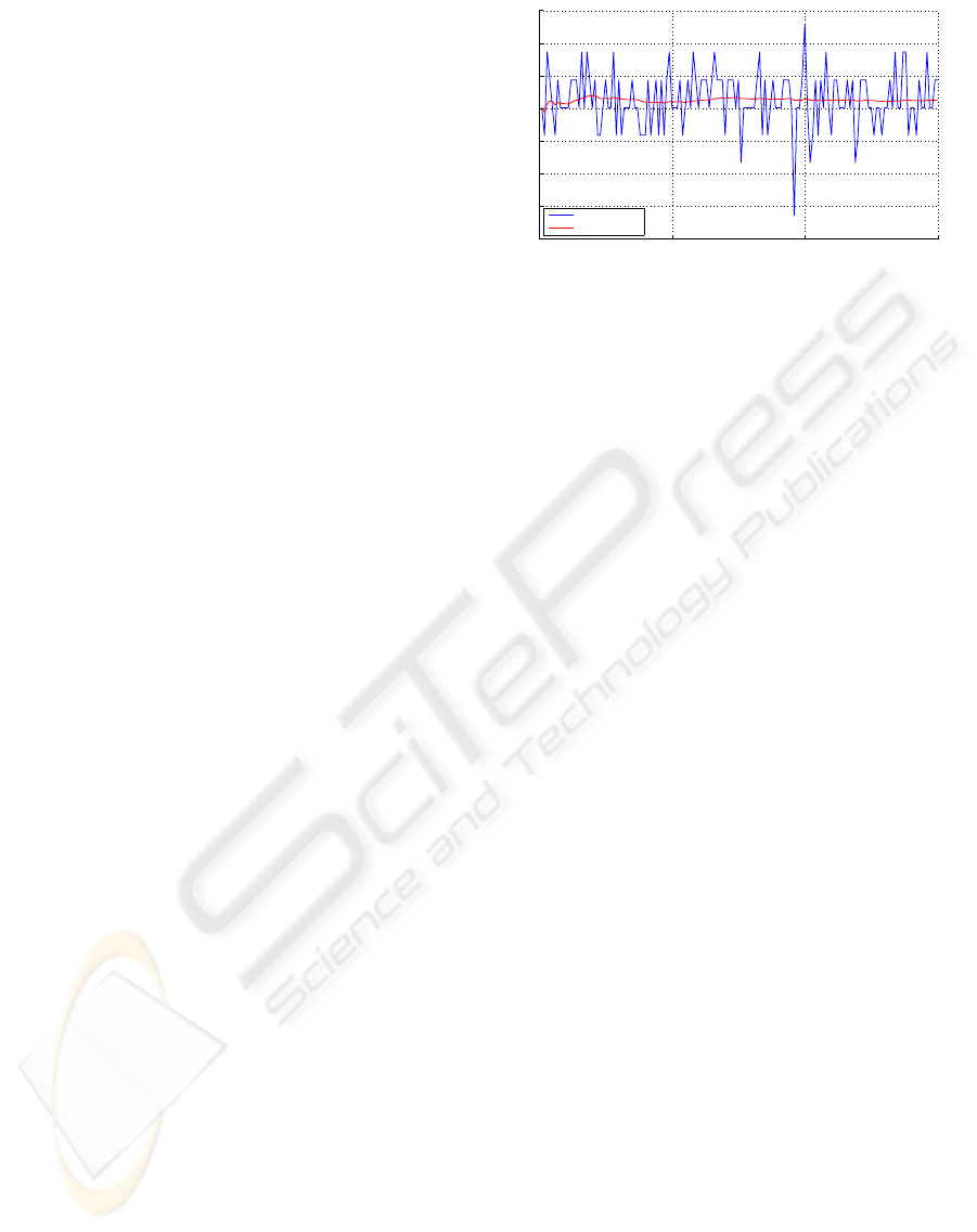
0 50 100 150

1530

1540

1550

1560

1570

1580

1590

1600

Sample index

Distance [cm]

Original

Kalman filtered

Figure 1: Kalman ﬁltered vs. non-ﬁltered depth values for

a single pixel in a static scene, q

= 0.001.

3.2.2 Free Space Marking

The occupancy grid is a direct top-down view of the

intensity image. If no occupied cell is found in a par-

ticular column, i.e. the direction of a ray from the

cameras focal point, all points in the real scene above

or below that ray are part of the free space up to the

vertical resolution of the occupancy grid.

4 EVALUATION

To evaluate the methods, a number of data sets have

been collected. Presented here is mainly one captured

on an electric vehicle with the camera at an angle of

◦

relative to the direction of travel, which is for-

ward.

4.1 State and Variance

To determine the effect on the state (the depth) of a

pixel in a stationary scene with a non-moving camera,

the ﬁrst 150 frames of a single pixel is compared to

its Kalman ﬁltered counterpart. Figure 1 shows this

for a depth of approximately 16 m. On average, the

variance was reduced from 52.14 to 4.10.

4.2 Density

The prediction property of the Kalman ﬁlter leads to

denser disparity maps, due to the accumulation of

measurements over time. Pixels which are predicted

for a given number of frames without being updated

with a new measurement are discarded to ensure stale

pixels do not degrade the occupancy grid. Note how

areas occluded in the raw disparity map (Figure 2a)

have a predicted depth in the Kalman ﬁltered map

(Figure 2d), leading to a denser disparity map than

without ego-motion.

VISAPP 2010 - International Conference on Computer Vision Theory and Applications

166

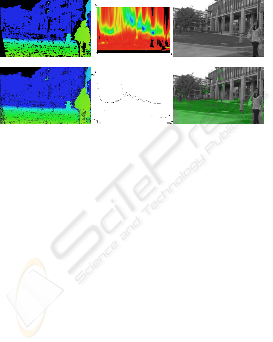
(a) Original disparity map.

1 px

500 px

0 m

57 m

(b) Full occupancy grid. (c) Left stereo image.

(d) Filtered disparity map. (e) Segmented. (f) Free space marked.

Figure 2: The steps undergone from stereo images to free space. They take place in the following order: (c) + right stereo

image → (a) → (d) → (b) → (e) → (f). In the last step, the depth of each pixel in (c) is looked up in (d), and if it is below the

line in (e) it is regarded as free space and marked green in (f).

4.3 Occupancy Grid and Free Space

Figure 2b is an example of an occupancygrid and Fig-

ure 2e of the resulting segmentation. The range of

depth represented by the occupancy grid is from 0 m

to 57 m. Also shown is the scene with (Figure 2f) and

without (Figure 2c) the free space marked.

5 CONCLUSIONS

We have shown how to estimate the free space in a

scene with a stereo camera. Iconic Kalman ﬁltering

of the disparity maps increases density and reduces

per-pixel variance (noise), leading to more accurate

stochastic occupancy grids and ultimately yielding a

more conﬁdent estimation of the occupancy of the

scene. For a more detailed review see (Høilund,

2009).

REFERENCES

Badino, H., Franke, U., and Mester, R. (2007). Free space

computation using stochastic occupancy grids and dy-

namic programming. Workshop on Dynamical Vision,

ICCV, Rio de Janeiro, Brazil.

Elfes, A. (1989). Using occupancy grids for mobile robot

perception and navigation. Computer, 22(6):46–57.

Høilund, C. (2009). Free space computation from stochas-

tic occupancy grids based on iconic Kalman ﬁltered

disparity maps. Master’s thesis, Aalborg University,

Laboratory of Computer Vision and Media Technol-

ogy, Denmark.

Kalman, R. E. (1960). A new approach to linear ﬁltering

and prediction problems. Transactions of the ASME–

Journal of Basic Engineering, 82(Series D).

Li, M., Hong, B., Cai, Z., Piao, S., and Huang, Q. (2008).

Novel indoor mobile robot navigation using monocu-

lar vision. Engineering Applications of Artiﬁcial In-

telligence, 21(3).

Mahalanobis, P. C. (1936). On the generalised distance in

statistics. In Proceedings National Institute of Sci-

ence, India, volume 2.

Matthies, L., Kanade, T., and Szeliski, R. (1989). Kalman

ﬁlter-based algorithms for estimating depth from im-

age sequences. International Journal of Computer Vi-

sion, 3(3):209–238.

Murray, D. and Little, J. (2000). Using real-time stereo vi-

sion for mobile robot navigation. Autonomous Robots,

8(2).

Trivedi, M. M., Gandhi, T., and McCall, J. (2007). Looking-

in and looking-out of a vehicle: Computer-vision-

based enhanced vehicle safety. Intelligent Transporta-

tion Systems, IEEE Transactions on, 8(1).

TYZX (2009). TYZX DeepSea Stereo Camera. [Online; ac-

cessed 20-November-09].

http://www.tyzx.com/

FREE SPACE COMPUTATION FROM STOCHASTIC OCCUPANCY GRIDS BASED ON ICONIC KALMAN

FILTERED DISPARITY MAPS

167