0BCHARACTERISTICS OF DEFINING HYPERPLANES OF
CONSTANT RETURNS TO SCALE TECHNOLOGY IN DEA
1BSevan Sohraiee
2BDepartment of Mathematics, Tehran North Branch, IAU, Darband st. Tehran, Iran
H
Keywords: Data envelopment analysis, Constant returns to scale technology, Defining hyperplanes.
Abstract: In this paper characteristics of defining hyperplanes of constant returns to scale technology in DEA have
been investigated. A defining hyperplane namely H is a type of hyperplane that with the elimination of H,
the production possibility set (PPS) will be enlarged (In this paper a defining hyperplane exactly is the full
dimensional efficient facet (FDEF) and may be found in Olesen and Peterson (1996, 2003)). The point of
view of some of the characteristics is conceptual and the interpretation of defining hyperplanes of constant
returns to scale technology can be achieved by these conceptual characteristics. However, some of the
characteristics are practical and one can easily utilize them in practice. Some parts of topology and convex
analysis have been considered to show the truth of characteristics.
1 INTRODUCTION
Data envelopment analysis (DEA) is a non-
parametric approach which was suggested by
Charnes et al. (1978) to measure the relative
efficiency of a decision making unit (DMU) and
provide DMUs with relative performance
assessment on multiple inputs and outputs. Based on
different essential properties and corresponding to
different characteristics of the production possibility
set (PPS) and production frontiers, different DEA
models, such as the CCR model, the BCC model and
the FDH model, have been introduced.
An important task of DEA is to identify the
returns to scale (RTS) of DMUs based on the
position of the supporting hyperplanes of efficient
frontier. Therefore, the investigation of different
types of hyperplanes of efficient frontier or PPS is
an important part of DEA.
No many papers in DEA have been written on
the subject of “investigation of efficient frontier”
and “characteristics of different types of
hyperplanes”. Finding of the piecewise linear
frontier of production function which identifies the
efficient frontier and efficient DMUs in DEA has
been investigated by Jahanshahloo et al. (2005), in
particular the aim of their study was to develop a
way to obtain efficient frontier by using 0-1 integer
programming, then by means of it, identification of
efficient DMUs and their returns to scale
characteristics. Also, searching of efficient frontier
in DEA, has been considered by Korhonen (1997).
Korhonen tried to provide the decision maker (DM)
an interactive method which allows him or her to
incorporate performance information in to the
efficient frontier analysis by enabling him or her to
make a free search on efficient frontier, furthermore,
Korhonen provided the DM all references of an
inefficient DMU, enabling him or her to choose the
most preferable unit as reference. Furthermore,
Jahanshahloo et al. (2007) suggested a way of
finding strong defining hyperplanes of production
possibility set in DEA, particularly their method is
based on the relation between efficient surfaces and
strong defining hyperplanes of production possibility
set. Also, Cooper et al. (2007) make it possible to
select the weights, obtained by the multiplier model
in DEA, associated with the facets of higher
dimension that a DMU generates, in particular their
method supplies model for locating facets of the
maximum possible dimension of the efficient
frontier. Furthermore, the construction of all DEA
efficient frontiers in generalized data envelopment
analysis (GDEA) has been discussed by Yu. et al.
(1996).
Almost in all of the abovementioned researches,
there is no investigation about the characteristics of
defining hyperplanes of production possibility set
that is so essential in DEA. In this paper, we have
65
Sohraiee S. (2010).
CHARACTERISTICS OF DEFINING HYPERPLANES OF CONSTANT RETURNS TO SCALE TECHNOLOGY IN DEA.
In Proceedings of the 7th International Conference on Informatics in Control, Automation and Robotics, pages 65-73
DOI: 10.5220/0002839400650073
Copyright
c
 SciTePress

presented some essential theorems in order to
identify the defining hyperplanes of constant returns
to scale (CRS) technology. These theorems enable
us to recognize whether a hyperplane obtained by
the optimal solution of the multiplier form of CCR
model is a defining hyperplane.
Furthermore, one of the most important task of
defining hyperplanes of production possibility set is
sensitivity analysis that enable us to determine the
amounts of perturbations of data that can be
tolerated by a DMU on efficient frontier before
becoming inefficient. Also, we can utilize the
concept defined in this paper in order to evaluate the
efficiency of DMUs by using the defining
hyperplanes of PPS, which efficient DMUs are on
them.
Some of the characteristics presented in this
paper are more conceptual, however others are more
practical. Furthermore, the conceptual point of view
of theorems presented in this paper, enable us to
interpret the characteristics of defining hyperplanes
of CRS technology. Although some of the theorems
are so practical and one can easily utilize them in
practice. Not only, the conceptual point of view of
theorems is essential and is so useful to
interpretation of defining hyperplanes of CRS
technology, but also the practical point of view of
theorems is a necessity and enable us to utilize the
characteristics in practice.
The aim of this paper is to use the conceptual
point of view of some parts of topology and convex
analysis and a combination of them with DEA to
present some conceptual and practical characteristics
in order to determine when a hyperplane of PPS is a
defining hyperplane. The main idea of this paper is
based on the geometrical interpretation of efficient
facets of the highest dimension of the frontier that
the DMU under assessment contributes to span. In
particular a defining hyperplane is a full dimensional
efficient facet (FDEF) and may be found in Olesen
and Peterson (2003). These geometrical
interpretations enable us to establish the presented
characteristics. Some of these characteristics are
conceptual that we will not be able to utilize them in
practice. Although, we use these conceptual
characteristics in order to establish some practical
characteristics that one may easily utilize them in
practice.
The sections of this paper are organized as
follows. In the next section, Section 2, we provide
additional background of our paper. In Section 3, we
give basic concepts of some parts of topology,
convex analysis and DEA models. Section 4
investigates the characteristics of defining
hyperplanes of constant returns to scale (CRS)
technology. In Section 5, we present an example to
illustrate the characteristics.
2 BACK GROUND
As previously noted, this paper is dealt with the
characteristics of defining hyperplanes of CRS
technology in DEA. These defining hyperplanes
play an important role in DEA as previously
mentioned.
In this paper, we restrict attention to geometrical
differences between defining hyperplanes of CRS
technology and those supporting hyperplanes of
CRS technology that are not defining. As we know,
these two kinds of hyperplanes play a crucial role in
DEA, since they are generally utilized to determine
different types of concepts such as efficiency, bench
mark DMUs, rates of substitution and
transformation, returns to scale, sensitivity analysis
and etc.
The main idea of this paper is based on
geometrical interpretation of defining hyperplanes of
CRS technology. In order to state a geometrical
characteristics of defining hyperplanes of CRS
technology, we use a combination of different kinds
of concepts such as interior points of a set, an
ε
-
neighborhood around a point and geometrical
interpretation of CRS technology efficient frontier to
state a specific relation between the dimension of
intersection of each defining hyperplanes with the
production possibility set (PPS) of CRS technology
that we use this characteristics to show the truth of
others stated characteristics.
Secondly, we utilize a model proposed by
Cooper et al. (2007) to determine a hyperplane that
is binding at the maximum number of extreme
efficient units. With utilizing the abovementioned
hyperplane namely
∗
H
, we define a created DMU
obtained by center of gravity of extreme efficient
units that the abovementioned hyperplane
∗
H
is
binding at them. Eventually, a set of feasible
directions obtained by connecting the created DMU
to each extreme efficient unit that the hyperplane
∗
H
is binding at them has been defined to present a
practical characteristic.
ICINCO 2010 - 7th International Conference on Informatics in Control, Automation and Robotics
66

3 THEORETICAL
CONSIDERATIONS
3.1 Some Basic Concepts of Topology
In this subsection we review some topological
properties of sets and some basic results from
convex analysis.
Definition 1. Given a point
n
Rx ∈
, a
−
ε
neighborhood around it is the set
{
}
ε
ε
<−= xyyxN )(
(1)
Definition 2. Let
X
be an arbitrary set in
n
R
.
x
is
said to be in the interior of
X
, denoted by Xint ,
if
XxN ⊂)(
ε
for some 0>
ε
.
Definition 3. Let
X
be an arbitrary set in
n
R
.
x
is
said to be in the boundary of
X
, denoted by
X
∂
,
if
)(xN
ε
contains at least one point in
X
and one
point not in
X
for every 0>
ε
.
Definition 4. A set
X
in
n
R
is called a convex set if
given any two points
1
x and
2
x in
X
then
Xxx ∈−+
21
)1(
λ
λ
for each
[]
1,0∈
λ
.
Definition 5. A point
x
in a convex set
X
is called
an extreme point of
X
, if
x
can not be represented
as a strict convex combination of two distinct points
in
X
.
Definition 6. A hyperplane
H
in
n
R
is a set of the
form
{
}
kpxx =
(2)
where
p
is a non-zero vector in
n
R
and k is a
scalar. Also,
p
is usually called the normal or the
gradient to the hyperplane.
Definition 7. A hyperplane divides
n
R
into two
regions, called half spaces. Hence two half spaces
+
H
and
−
H
may be defined in the following
manner:
{}
kpxxH ≥=
+
(3)
{}
kpxxH ≤=
−
(4)
where
p
is a non-zero vector in
n
R
and k is a
scalar. Also,
−+
= HHH ∩
(5)
Definition 8. A polyhedral set or polyhedron is the
intersection of a finite number of halfspaces. A
bounded polyhedral set is called a polytope.
Suppose that the polyhedral set under discussion
in the following definitions has the form
{
}
0, ≥≤= xbAxxX
(6)
where
A
is nm
×
and b is an m -vector. The
hyperplanes associated with the
)( nm +
defining
halfspaces
mibxax
ii
,...,1},{ =≤
(7)
And
njxex
j
,...,1},0{ =≥
(8)
are called defining hyperplanes of
X
.
Definition 9. Let
Xx
∈
. A constraint
ll
bxa ≤
is
binding, or tight, or active, at
Xx ∈ , if
ll
bxa =
(9)
Definition 10. A hyperplane
H
is a supporting
hyperplane of
X
, if
Φ
≠
XH ∩ &
)(
−+
⊆⊆ HXorHX
(10)
Definition 11. The set of points in
X
that
correspond to some non-empty of binding defining
hyperplanes of
X
are called faces of
X
. Given any
face
F
of
X
if
)(Fr
is the maximum number of
linearly independent defining hyperplanes binding at
all points feasible to
F
, then the dimension of
F
,
denoted by
)dim(F
, is equal to
)(Frn −
.
Also, the highest dimensional face of
X
is of
dimension
1)dim(
−
X
and it is called a facet of
X
.
3.2 DEA Background
Assume that we have n DMUs each consuming m
inputs and producing
s outputs. Let be an
CHARACTERISTICS OF DEFINING HYPERPLANES OF CONSTANT RETURNS TO SCALE TECHNOLOGY IN
DEA
67

)( nm×
-matrix and be a
)( ns ×
-matrix
consisting of non-negative elements, containing
observed input and output measures for the DMUs,
respectively. We denote by
njXX
jj
,...,1,0,0 =≠≥
(the jth column of
) the vector of inputs consumed by DMU
j
. A
similar notation is used for outputs.
The traditional CCR models, as introduced by
Charnes et al. (1978) are fractional linear programs,
which can easily be formulated and as linear
programs. Those models are so-called constant
returns to scale (CRS) models. Later Banker et al.
(1984) developed the so-called BCC models with
variable returns to scale (VRS).
The CCR and BCC models are the basic model
types in DEA. Those basic models can be presented
in a primal or dual form. The usage of primal and
dual varies in the literature, and it is more
straightforward to call them multiplier and
envelopment models, respectively. The multiplier
model provides information on the weights of inputs
and outputs. The weights are interpreted as prices in
many applications. The envelopment models provide
the user with information on the lacks of outputs and
the surplus of inputs of a unit. Also, the envelopment
model characterizes the reference set for the units.
Moreover, the production possibility set (PPS) of
CCR and BCC models can be interpreted from the
structure of envelopment models. Since, we are
interested in CCR models in this paper, we represent
the PPS of constant returns to scale (CRS)
technology in the following manner:
⎪
⎭
⎪
⎬
⎫
⎪
⎩
⎪
⎨
⎧
≥
≥≤=
=
0
,,),(
λ
λλ
YXYXZ
T
T
c
(11)
Based on the PPS of CRS technology the
envelopment form of CCR model is in the following
manner:
θ
Min
.0
..
≥
≥
≤
λ
λ
θλ
o
o
Y
XtS
(12)
The multiplier form of model CCR based on the
dual of model (12) is as follows:
o
T
YUMax
(13)
0,0
,...,1,0
1..
≥≥
=≤−
=
VU
njXVYU
XVtS
j
T
j
T
o
T
(13.1)
(13.2)
We know that in the optimal solution
),(
∗∗
VU
of model (13), at least one constraints of
(13.2) is binding. Also, it is easy to show, this
optimal solution
),(
∗∗
VU
is the normal vector of a
supporting hyperplane
{
}
0),( =−=
∗∗∗
XVYUYXH
TTT
(14)
which, supports
c
T
constructed by observed
data.
Definition 12. DMU
o
is an extreme efficient unit if
in the evaluation of DMU
o
, the optimal solution of
model (12) is unique and
0,1 ==
∗
≠
∗
ojo
λλ
(15)
Also, the indices of all extreme efficient units is
denoted by
{
}
unitefficientextremeanisDMUjE
j
=
(16)
We know that
c
T
is the intersection of some
hyperplanes. We call some of these hyperplanes as
defining hyperplanes if with the elimination of these
hyperplanes,
c
T
will be enlarged.
Definition 13. A hyperplane
H
is a defining
hyperplane of
c
T
if with the elimination of
H
,
c
T
will be enlarged (A defining hyperplane used in this
paper exactly is FDEF defined by Olesen and
Peterson (2003)).
4 CHARACTERISTICS OF
DEFINING HYPERPLANES OF
CRS TECHNOLOGY
In this section, we present some essential theorems
in order to recognize all defining hyperplanes of
c
T
.
In these theorems some important characteristics of
defining hyperplanes of
c
T
have been identified.
These theorems enable us to recognize when a
hyperplane is a defining hyperplane of
c
T
.
Therefore, using these theorems one will be able to
recognize any defining hyperplanes of
c
T
which
was not possible before. As mentioned in previous
ICINCO 2010 - 7th International Conference on Informatics in Control, Automation and Robotics
68

sections, if
),(
∗∗
VU
is an optimal solution of the
multiplier model of CRS technology (13), then
}0),{( =−
∗∗
XVYUYX
TT
(17)
will be a supporting hyperplane of
c
T
. Assume that
{
}
Kt
XVYUYXH
T
t
T
t
T
t
,...,1
,0),(
=
=−=
(18)
are all defining hyperplanes of
c
T
which we are
interested in. Also consider two defining half-spaces
{
}
0),( ≥−=
+
XVYUYXH
T
t
T
t
T
t
(19)
and
{
}
0),( ≤−=
−
XVYUYXH
T
t
T
t
T
t
(20)
obtained by hyperplane
t
H
for each
Kt ,...,1=
.
With out loss of generality, we can assume that
c
T
is the intersection of all defining half-spaces
KtH
t
,...,1, =
−
in the following manner:
−
=
=
t
K
tc
HT
1
∩
(21)
Theorem 1. The hyperplane
H
is a defining
hyperplane of
c
T
if and only if the dimension of
)( HT
c
∩
equals 1
−
+ sm .
Proof. Assume that the dimension of
)( HT
c
∩
equals
1−+ sm . On one hand, since,
Φ≠HT
c
∩
, we can find a point such as
HTYXZ
c
T
∩∈= ),( for which there exists a
)1( −+ sm
dimensional −
ε
neighborhood
HTZN
c
∩⊆)(
ε
. On the other hand,
T
YXZ ),(=
is a point contained in
c
T
for which,
only one hyperplane such as
H
is binding.
Therefore, with the elimination of half-space
−
H
obtained by hyperplane
H
from
c
T
(without
loss of generality assume that
−
⊆ HT
c
), the point
T
YXZ ),(=
will be an interior point of
c
T
′
(
c
T
′
is
the set obtained by the elimination of half-
space
−
H
from
c
T
). Note that
cc
TT
′
⊆
. Since,
T
YXZ ),(=
is an interior point of
c
T
′
, therefore,
there exists an
,0>
ε
for which,
c
TZN
′
⊆)(
ε
.
Also, since
c
T
TYXZ ∂∈= ),(
, each
)(ZN
ε
contains at least one point in
c
T
and one
point not in
c
T
for every 0>
ε
. Now, assume that
this neighborhood is
)(ZN
ε
. Thus, there exists a
point such as
o
Z
for which
)(ZNZ
o ε
∈
and
co
TZ
∉
. This shows that
co
TZ
′
∈
and
co
TZ
∉
.
Consequently,
cc
TT
′
⊂
and therefore, it means that
with the elimination of half-space
−
H
from
c
T
,
c
T
has been enlarged. Thus,
H
is a defining hyperplane
of
c
T
.
To show the converse, assume that the
hyperplane
H
is a defining hyperplane of
c
T
. It is
obvious that the dimension of each hyperplane such
as
H
in
sm
R
+
such as
c
T
is equal to
)1(
−
+ sm
.
Since,
H
is a defining hyperplane of
c
T
therefore,
there exists a point such as
T
YXZ ),(=
in the
interior of
HT
c
∩
. Now, with the elimination of
half-space
−
H
from
c
T
, we will encounter with a
set called
c
T
′
(
cc
TT
′
⊂
). Since,
)int(),( HTYXZ
c
T
∩∈=
, thus,
T
YXZ ),(=
will be an
interior point of
c
T
′
. This implies that there exists an
0>
ε
for which the
−+ )( sm
dimensional
c
TZN
′
⊂)(
ε
. Now, it is trivial that
HZN ∩)(
ε
is
−
−
+
)1( sm
dimensional and this
implies that
HT
c
∩
is
−−+ )1( sm
dimensional.
This completes the proof. 
Theorem 1 shows a characteristic of defining
hyperplane of
c
T
. In order to simplify and find
more simple methods for introduction of defining
hyperplanes of
c
T
, we need to use the following
model that has been introduced by Cooper et al.
(2007) with some minor modification:
CHARACTERISTICS OF DEFINING HYPERPLANES OF CONSTANT RETURNS TO SCALE TECHNOLOGY IN
DEA
69

∑
=
n
j
j
lMin
1
{}
.,0,0,0
,1,0
,0
,0
1
1..
EjtVU
Ejl
EjMlt
EjtXVYU
XV
YUtS
j
j
jj
jj
T
j
T
P
T
P
T
∈≥≥≥
∈∈
∈≤−
∈=+−
=
=
(22)
Where
M
is sufficiently large positive number and
E
is the set of indices of all extreme efficient
DMU’s defined in previous sections.
Since,
Φ≠
E
, thus model (22) finds a
hyperplane which, is binding, at the maximum
number of extreme efficient units.
Assume that
),,,(
∗∗∗∗
LTVU
,
),...,(
1
∗∗∗
=
E
ttT
),...,(
1
∗∗∗
=
E
llL
(23
)
is an optimal solution of model (22). We define the
hyperplane
∗
H
in the following manner:
{
}
0),( =
∗
−
∗
=
∗
X
T
VY
T
U
T
YXH
(24)
The following theorem emphasizes the existence
of a defining hyperplane of
c
T
at each extreme
efficient unit.
Theorem 2. There exists at least one defining
hyperplane of
c
T
such as H for each
Ej
∈
, for
which,
HYXZ
T
jjj
∈= ),(
.
Proof. As we know,
−
=
=
t
K
tc
HT
1
∩
. To the
contrary of the desired result, suppose that there is
no defining hyperplane of
c
T
which is binding
at
EjYXZ
T
jjj
∈= ,),(
. Therefore,
KtHYXZ
tjjj
,...,1),(int),( =∈=
−
.
Consequently,
)(int),(
cjjj
TYXZ ∈=
, which is in
contradiction with
Ej ∈
. This completes the
proof. 
In order to improve the conditions under which
one can more easily identify the defining
hyperplanes of
c
T
and present more practical
characteristics of determining defining hyperplanes
of
c
T
, we define a set based on the optimal solution
of model (22) as follows:
{
}
)22(,0 intjE
j
==
∗∗
(25)
The following theorem, shows that,
∗
E
is not
vacuous.
Theorem 3.
Φ
≠
∗
E
.
Proof.
The proof is obvious and omitted. 
The improvement of conditions and characteristics
of determining defining hyperplanes of
c
T
made us
define a created DMU in the following manner:
∑
∗
∈
∗
∗∗∗
==
Ej
T
jj
T
YX
E
YXZ ),(
1
),(
(26)
Particularly,
T
YXZ ),(
∗∗∗
=
is the center of
gravity of extreme efficient units for which, the
hyperplane
∗
H
(defined based on the optimal
solution of model (22)) is binding. The following
theorem states that,
T
YXZ ),(
∗∗∗
=
is in
boundary of
c
T
.
Theorem 4.
c
T
TYXZ ∂∈=
∗∗∗
),(
.
Proof. Noting theorem 3, we have
Φ≠
∗
E
.
Therefore,
∗
H
defined in (24) is a supporting
hyperplane of
c
T
. Since,
c
T
is a convex set
therefore,
c
T
TYXZ ∈=
∗∗∗
),(
. Also, we have
∑
∑∑
∗
∗∗
∈
∗∗
∗
∈
∗
∗
∈
∗
∗
∗∗∗∗
=−
=−
=−
Ej
jj
Ej
j
Ej
j
XVYU
E
X
E
VY
E
U
XVYU
0)(
1
)
1
()
1
(
(27)
This shows that the defining hyperplane
∗
H
is
binding at
c
T
TYXZ ∈=
∗∗∗
),(
and it means that
c
T
TYXZ ∂∈=
∗∗∗
),(
and this completes the
proof. 
Theorem 5. If the optimal solution of model (13) in
the evaluation of created unit
T
YXZ ),(
∗∗∗
=
is
unique then the hyperplane
∗
H
will be a defining
hyperplane of
c
T
.
ICINCO 2010 - 7th International Conference on Informatics in Control, Automation and Robotics
70

Proof. Consider the following model, which is the
multiplier form of CCR model based on the set
E
when unit
T
YXZ ),(
∗∗∗
=
is under evaluation:
∗
YUMax
T
.0,0
1
0
,0..
≥≥
=
≤−
∈≤−
∗
∗∗
VU
XV
XVYU
EjXVYUtS
T
TT
j
T
j
T
(28)
Assume that model (28) has unique optimal
solution
),( VU
. Define,
{
}
0),( =−= XVYUYXH
TT
(29)
It is obvious that
0=−
∗∗
XVYU
TT
and
H
is
the only supporting hyperplane of
c
T
at
T
YXZ ),(
∗∗∗
=
. Therefore, we can define a face of
c
T
for which,
T
YXZ ),(
∗∗∗
=
is on it as follows:
c
THF ∩=
It is trivial that
F
is the only face contained
T
YXZ ),(
∗∗∗
=
, therefore, the dimension of
F
equals to
1−+ sm and this means that the
dimension of
c
TH ∩
equals to 1
−
+
sm .
Therefore, considering Theorem 1,
H
is a defining
hyperplane of
c
T
. Note that
H
is equivalent to
∗
H
and this means that
∗
H
is a defining hyperplane of
c
T
, thus the proof is complete. 
To simplify and improve better recognition of
defining hyperplanes of
c
T
, we utilize the following
definition of feasible directions constructed by
connecting
T
YXZ ),(
∗∗∗
=
to each extreme
efficient unit that
∗
H
is binding at them:
⎪
⎭
⎪
⎬
⎫
⎪
⎩
⎪
⎨
⎧
∈
−=
=
∗
∗∗
Ej
YXYXd
dD
TT
jjj
j
,),(),(
(30)
Theorem 6. If the dimension of D equals to
1−+ sm then
∗
H
is a defining hyperplane of
c
T
.
Proof. Noting that
c
T
TYXZ ∈=
∗∗∗
),(
,
c
T
jjj
TYXZ ∈= ),(
for each
∗
∈ Ej
and
c
T
is a
convex set, we have
(
)
cj
TZZZ ∈−+
∗∗
λ
for each
∗
∈ Ej
and
[
] 1,0
∈
λ
. Also, since
∗∗∗∗
∈= HYXZ
T
),(
,
∗
∈= HYXZ
T
jjj
),(
for
each
∗
∈ Ej
and
∗
H
is a convex set,
therefore
(
)
∗∗∗
∈−+ HZZZ
j
λ
for each
∗
∈ Ej
and
[
] 1,0
∈
λ
. Thus, these imply that
(
)
∗∗∗
∈−+ HTZZZ
cj
∩ λ
for each
∗
∈ Ej
and
[
] 1,0
∈
λ
. Therefore, since, the dimension of
D
equals to
1
−
+
sm
, thus we have 1
−
+ sm
independent feasible direction at
∗
Z
in
∗
HT
c
∩
.
This implies that the dimension of
∗
HT
c
∩
equals
to
1
−
+
sm
and by theorem 1,
∗
H
is a defining
hyperplane of
c
T
. Therefore the proof is
complete.
5 ILLUSTRATIVE EXAMPLE
In order to illustrate the characteristics of Theorems,
we present a numerical example with the data set as
in table 1. The CRS technology based on the data set
in Table 1, has been illustrated in Fig. 1. This figure
can be viewed as representing a section at a given
output level, say
1
=
y
, of the PPS generated two
DMUs (A and B) that use two inputs and produce
the same quantity of output (
1=y
). The optimal
solutions of (12) when assessing the efficiency of
the extreme efficient DMU A or DMU B correspond
to the coefficients of the supporting hyperplanes at
A or B, which pass through origin. Model (22) then
selects the hyperplane represented with a dark solid
line conneting as distinct from the ones represented
by the lighter dotted lines. The first one is obviously
preferable to the latter because it is supported by two
units (A and B) instead of by only one (A) or one
(B). Moreover, in this particular case, this also
means that it contains a FDEF of the frontier that
DMU A and DMU B contribute to generate.
CHARACTERISTICS OF DEFINING HYPERPLANES OF CONSTANT RETURNS TO SCALE TECHNOLOGY IN
DEA
71

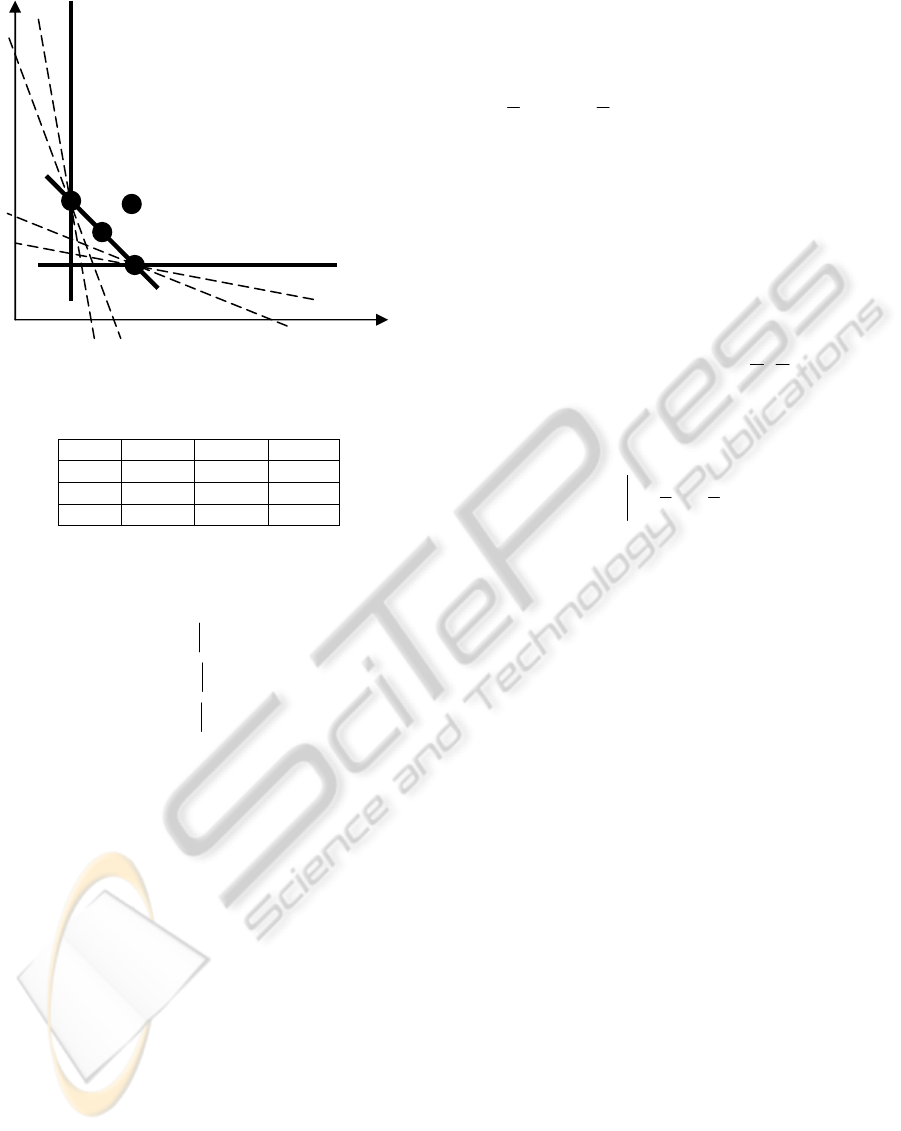
X
2
A C
Z*
B
X
1
Figure 1: The graph of example.
3BTable 1: Data set.
DMU Input 1 Input 2 Output
A 1 2 1
B 2 1 1
C 2 2 1
It is obvious that the defining hyperplanes of
c
T
are
in the following manner:
{
}
022),,(
1211
=−= xyyxxH
T
{
}
03),,(
21212
=−−= xxyyxxH
T
{
}
022),,(
2213
=−= xyyxxH
T
We can see that
2)dim(
1
=
HT
c
∩
,
2)dim(
2
=HT
c
∩
and
2)dim(
3
=HT
c
∩
as it
has been shown in Theorem 1. Therefore, the
condition of Theorem 1,
1)dim(
−
+= smHT
tc
∩
has been satisfied and
this shows the truth of Theorem 1.
The optimal solution of model (3) shows that
{}
2,1=E . As stated in Theorem 2, the
hyperplanes
1
H and
2
H are two defining
hyperplanes of
c
T
associated with
ADMU
and
the hyperplanes
2
H and
3
H
are two defining
hyperplanes of
c
T
associated with
BDMU
.
These show the truth of Theorem 2.
If we solve the model (22) it will be obtained that
{}
2,1=
∗
E
and this shows the truth of Theorem 3.
If we utilize the relation (26) we will encounter with
a created DMU,
() ()( )
TTT
T
YXZ
1,5.1,5.11,1,2
2
1
1,2,1
2
1
),(
=+=
=
∗∗∗
(31)
which has been shown in Fig. 1. It is trivial that the
hyperplane
2
H
is binding at
()
T
Z 1,5.1,5.1=
∗
.
Consequently,
(
)
c
T
TZ ∂∈=
∗
1,5.1,5.1 and this
shows the truth of Theorem 4.
If we solve model (11) associated with created
DMU,
(
)
T
Z 1,5.1,5.1=
∗
, we will obtain a unique
optimal solution
(
)
⎟
⎠
⎞
⎜
⎝
⎛
=
∗
∗
∗
1,
3
1
,
3
1
,,
21
vvu . Now,
based on the optimal solution of model (28), the
hyperplane
∗
H
will be in the following manner:
⎭
⎬
⎫
⎩
⎨
⎧
=−−=
∗
0
3
1
3
1
),,(
2121
xxyyxxH
T
(32)
that is exactly the hyperplane
2
H . This shows the
truth of Theorem 5.
The set
D
as stated in (13) is as follows:
()
()
⎪
⎭
⎪
⎬
⎫
⎪
⎩
⎪
⎨
⎧
−=
−=
=
T
T
d
d
D
0,5.0,5.0
,0,5.0,5.0
2
1
(33)
It is obvious that
1)dim( =D
. Since,
∗
H
is a
defining hyperplane of
c
T
, the converse of Theorem
6 does not hold and this shows that Theorem 6 is
only a sufficient condition.
6 CONCLUSIONS
In this paper, some parts of topology and convex
analysis have been utilized in order to state some
characteristics of defining hyperplanes of CRS
technology in DEA. These characteristics enable us
to recognize whether a hyperplane obtained by the
optimal solution of multiplier form of CCR model is
a defining hyperplane. Some of the characteristics
are conceptual and some of them can be easily
utilized in practice. An illustrative example has been
considered, in order to show the truth of
characteristics stated in this paper.
We suggest as a future research, introduction of
an algorithm to recognize all defining hyperplanes of
ICINCO 2010 - 7th International Conference on Informatics in Control, Automation and Robotics
72

CRS technology based on characteristics presented
in this paper. Also, we look for similar
characteristics in the case of variable returns to scale
technology as a future research.
REFERENCES
Banker, R. D., Charnes, A., Cooper, W. W., 1984. Some
models for estimating technical and scale
inefficiencies in data envelopment analysis. 30 1078-
1092, Management Science.
Charnes, A., Cooper, W. W., Rhodes, E., 1978. Measuring
the efficiency of decision making units, 2 429-444.
European Journal of Operational Research.
Cooper, W. W., Ruiz, J. L., Inmaculada Sirvent, 2007.
Choosing weights from alternative optimal solutions
of dual multiplier models in DEA, 180 443-458.
European Journal of Operational Research.
Jahanshahloo, G. R., Hosseinzadeh Lotfi, F., Zhiani Rezai,
H., Rezai Balf, F., 2007. Finding strong defining
hyperplanes of Production Possibility Set, 177 42-54.
European Journal of Operational Research.
Jahanshahloo, G. R., Hosseinzadeh Lotfi, F.,
Zohrehbandian, M., 2005. Finding the piecewise linear
frontier production function in Data Envelopment
Analysis, 163 483-488. Applied Mathematics and
Computation.
Korhonen, P., 1997. Searching the efficient frontier in
Data Envelopment Analysis, IR-79-97. IIASA.
Olesen, O., Petersen, N. C., 1996. Indicators of ill-
conditioned data sets and model misspecification in
data envelopment analysis: An extended facet
approach,42 205-219. Management Science.
Olesen, O., Petersen, N. C., 1996. Identification and use of
efficient faces facets in DEA, 20 323-360. Journal of
Productivity Analysis.
Yu, G., Wei, Q., Brockett, P., Zhou, L., 1996.
Construction of all DEA efficient surfaces of
Production Possibility Set under the generalized Data
Envelopment Analysis model, 95 491-510. European
Journal of Operational Research.
CHARACTERISTICS OF DEFINING HYPERPLANES OF CONSTANT RETURNS TO SCALE TECHNOLOGY IN
DEA
73