
HOMOTHETIC APPROXIMATIONS FOR STOCHASTIC PN
Dimitri Lefebvre
GREAH – University Le Havre, France
Keywords: Stochastic Petri Nets, Continuous Petri Nets, Fluidification, Steady State, Reliability Analysis.
Abstract: Reliability analysis is often based on stochastic discrete event models like stochastic Petri nets. For complex
dynamical systems with numerous components, analytical expressions of the steady state are tedious to
work out because of the combinatory explosion with discrete models. For this reason, fluidification is an
interesting alternative to estimate the asymptotic behaviour of stochastic processes with continuous Petri
nets. Unfortunately, the asymptotic mean marking of stochastic and continuous Petri nets are mainly often
different. This paper proposes a geometric approach that leads to a homothetic approximation of the
stochastic steady state in specific regions of the marking space.
1 INTRODUCTION
Reliability analysis is a major challenge to improve
the safety of industrial processes. For complex
dynamical systems with numerous interdependent
components, such studies are mainly based on
stochastic discrete event models like Markov models
(Rausand et al., 2004) or stochastic Petri nets (SPNs)
(Molloy, 1982). Such models are mathematically
well founded and lead either to analytical results or
numerical simulations. But in case of large systems,
the combinatory explosion limits their use. In this
context, fluidification can be discussed as a
relaxation method.
This paper is about the approximation of the
SPNs asymptotic mean markings and average
throughputs by mean of continuous Petri nets
(CPNs) under infinite server semantic (Vazquez et
al., 2008; Lefebvre et al., 2009). The limits of the
fluidification of SPNs are discussed according to the
partition in regions of the reachability state space. A
characterization of the regions is proposed that leads
to a homothetic approximation of the stochastic
steady state. The proposed results are not
constructive but concern the existence of solutions.
They may be helpful to investigate the properties of
a considered SPN and they may lead for example to
the design of observers or controllers for stochastic
processes.
2 FLUIDIFICATION OF SPN
2.1 Stochastic Petri Nets
A Petri net (PN) is defined as <P, T, W
PR
, W
PO
>
where P = {P
i
} is a set of n places and T = {T
j
} is a
set of q transitions, W = W
PO
– W
PR
(Z)
nq
is the
incidence matrix, M(t) is the PN marking vector and
M
I
the PN initial marking (David et al., 1992).
Depending on the incidence matrix, PNs may have
P-semiflows. A P-semiflows y (Z
+
)
n
is a non-zero
solution of equation y
T
.W = 0. Let define Y = {y
1
,...,
y
h
} as a basis of W
T
kernel, composed of h minimal
P-semiflows. For simplicity, the basis Y will be
represented as a matrix Y (Z
+
)
n x h
that satisfies (1):
Y
T
.M(t) = Y
T
.M
I
= C, t 0 (1)
Let define, for each minimal P-semiflow y
i
Y, its
support as the subset P(y
i
) P of places that belong
to the corresponding marking invariant. For each
P(y
i
) it is possible to select a single place and to
recover the marking of this place from the marking
of the other places in P(y
i
). Let define as a
consequence the subset P
2
P of h places whose
markings may be recovered from Y, and the subset
P
1
P of n - h other places. The permutation matrix
D defined according to P
1
and P
2
leads to the
marking M’ = ((M’
1
)
T
(M’
2
)
T
)
T
= D.M .
A stochastic Petri net (SPN) is a timed PN whose
transitions firing periods are characterized a firing
364
Lefebvre D. (2010).
HOMOTHETIC APPROXIMATIONS FOR STOCHASTIC PN.
In Proceedings of the 7th International Conference on Informatics in Control, Automation and Robotics, pages 364-367
DOI: 10.5220/0002918003640367
Copyright
c
SciTePress

rate vector µ = (µ
j
) (R
+
)
q
(Molloy, 1982). The
marking and mean marking vectors of a SPN at time
t will be referred as M
s
(t) and MM
s
(t). The SPNs
considered in this paper are bounded, reinitialisable,
with infinite server semantic, race policy and
resampling memory. As a consequence, the
considered SPNs have a reachability graph with a
finite number N of states and their marking process
is mapped into a Markov model with state space
isomorphic to the reachability graph (Bobbio et al.,
1998). The Markov model has an asymptotic state
propability vector
ss
= (
ss k
) [0, 1]
1 x N
and the
asymptotic mean marking M
mms
of SPNs depends
from
ss
:
.
,1,..,
,…,
(2)
2.2 Continuous Petri Nets and Regions
CPNs have been developed in order to provide
continuous approximations of the discrete
behaviours of PNs (David et al., 1992; Silva and
Recalde, 2004). A CPN is defined as < PN, X
max
>
where PN is a Petri nets and X
max
= diag(x
max j
)
(R
+
)
qxq
is the diagonal matrix of maximal firing
speeds x
max j
, j = 1,…q. M
c
(t) is the marking vector
and X
c
(t) = (x
cj
(t)) (R
+
)
q
is the firing speeds vector
that satisfy dM
c
(t) / dt = W.X
c
(t). For CPNs with
infinite server semantic, X
c
(t) depends continuously
on the marking of the places according to x
cj
(t) =
x
max j
. min (m
k
(t) / w
PR
kj
), for all P
k
°T
j
, where °T
j
stands for the set of T
j
upstream places. A marked
CPN has a steady state if the marking vector M
c
(t)
tends to a finite limit M
mmc
in long run.
According to the function “min(.)”, the marking
space of CPNs is divided into K regions A
k
(eventually empty) with K = |°T
1
| x… x |°T
q
|. Each
region A
k
is defined by its PT-set (Julvez et al.
2005) defined according to (3):
PT-set(A
k
) = {(
P
i
,
T
j
) s.t.
M
c
(t) A
k
,
x
c
j
(t) = x
max
j
(t).m
ci
(t)/w
PR
i
j
}
(3)
The place P
i
such that i = argmin (m
k
(t) / w
PR
kj
)
for all P
k
°T
j
is the critical place for transition T
j
at
time t. A constraint matrix A
k
= (a
k
ij
) (R
+
)
q x n
, k =
1,…,K, i = 1,..., q and j = 1,..., n is defined for each
region A
k
according to the corresponding PT-set: a
k
ij
= 1/w
PR
ji
if (P
i
, T
j
) PT-set(A
k
) and a
k
ij
= 0
elsewhere. For each region A
k
, equation (4) holds:
M
c
(t)
A
k
, dM
c
(t) / dt = W. X
max
.
A
k
.M
c
(t) (4)
Definition: A region A
k
is critical if there exists two
transitions T
j
and T
k
that have the same critical place
P
i
in region A
k
.
Proposition 1: Marking M
c
A
k
iff M
c
satisfies (5):
.
0
0
C
C
(5)
with In and the identity matrix of size n and:
…
.
(6)
Proof: Equation (5) results from the definition of
PT-sets and P-semiflows of the PN. The equation
-I
n
.M
c
0 stands for the positivity of the marking.
The equation A(k).M
c
= 0 defines the region borders
according to the “min” functions. Finally, the
equation Y
T
.M
C
C and -Y
T
.M
C
-C result from the
P-semiflows.
2.3 Continuous Approximation of
SPNs
Numerous structural and behavioural properties are
not preserved with fluidification (Silva and Recalde
2004). The average throughput and mean marking of
a CPN are mainly not identical to the ones of a
discrete PN (Julvez et al., 2005, Lefebvre et al.,
2009). Concerning SPNs, the steady state is mainly
often different from the one of a CPN with same
parameters (x
maxj
=
j
j = 1,...,q). The asymptotic
mean markings of SPNs can be approximated with
the steady state of CPNs if all transitions remain
enabled with degree at least 1 in long run and the
marking vector does not leave the region of initial
marking in long run (Vasquez et al, 2008). These
conditions limit strongly the interest of
fluidification. In our preceding works, we have
investigated the limit of fluidification for the
approximation of SPNs. CPNs with a modified set of
maximal firing speed can be used to approximate the
mean marking in non critical regions (Lefebvre and
Leclercq 2010). In the next section, we continue this
investigation for critical regions.
3 HOMOTHETIC ESTIMATION
Let consider the problem to reach Mmms when
Mmms Ai (eventually critical) and MI Ak (non
critical) with Ai Ak. The proposition 2 provides
conditions to work out admissible but partial
HOMOTHETIC APPROXIMATIONS FOR STOCHASTIC PN
365
homothetic transformations of ratio such that
(.(M’mms1)T (M”
mms2
)
T
)
T
A
k
. Then a CPN with
modified constant maximal firing speeds (x
maxj
j
j
= 1,...,q) is worked out with proposition 3. This CPN
approximates
.M’
mms1
.
Proposition 2: Let define M’
mms
= D.M
mms
and
M”
mms2
such that the Y
T
.(.(M’
mms1
)
T
(M”
mms2
)
T
)
T
=
C. The condition (.(M’
mms1
)
T
(M”
mms2
)
T
)
T
A
k
holds if
satisfies (7):
Y
T
Y
T
.D
.
.
"
0
0
(7)
Proof: Proposition 2 results from proposition 1 by
replacing M
c
by D
-1
.D.M
c
and by considering the
partial homothetic transformations of ratio
.
Proposition 2 characterises the intersection of the
region A
k
and the direction M
mms
.
Proposition 3: Consider a SPN with M
I
A
k
(non
critical) and M
mms
A
i
(eventually critical) with A
i
A
k
. Let define the CPN with same structure and
initial marking. M
c
(t) tends asymptotically to M
mmc
such that M’
mmc1
=
.M’
mms1
if there exist X
max
such
that M
c
(t) satisfies the proposition 1 for all t 0 and
equation (8) holds:
W.X
.A
.D
.
.
"
0
(8)
Proof: Proposition 3 results from the steady state
solution of equation (4) and from the partial
homothetic transformations of ratio
..
The propositions 2 and 3 lead to a 4-stages
algorithm for estimating Mmms in critical regions.
Work out the transformation matrix D.
List the conditions to be satisfied by , so that
the partial homothetic transformation of Mmms and
MI are in the same non critical region.
Work out the modified constant firing speeds
that drive Mc(t) to Mmmc st M’mmc1 = .M’mms1.
Recover the asymptotic stochastic mean marking
Mmms with (1).
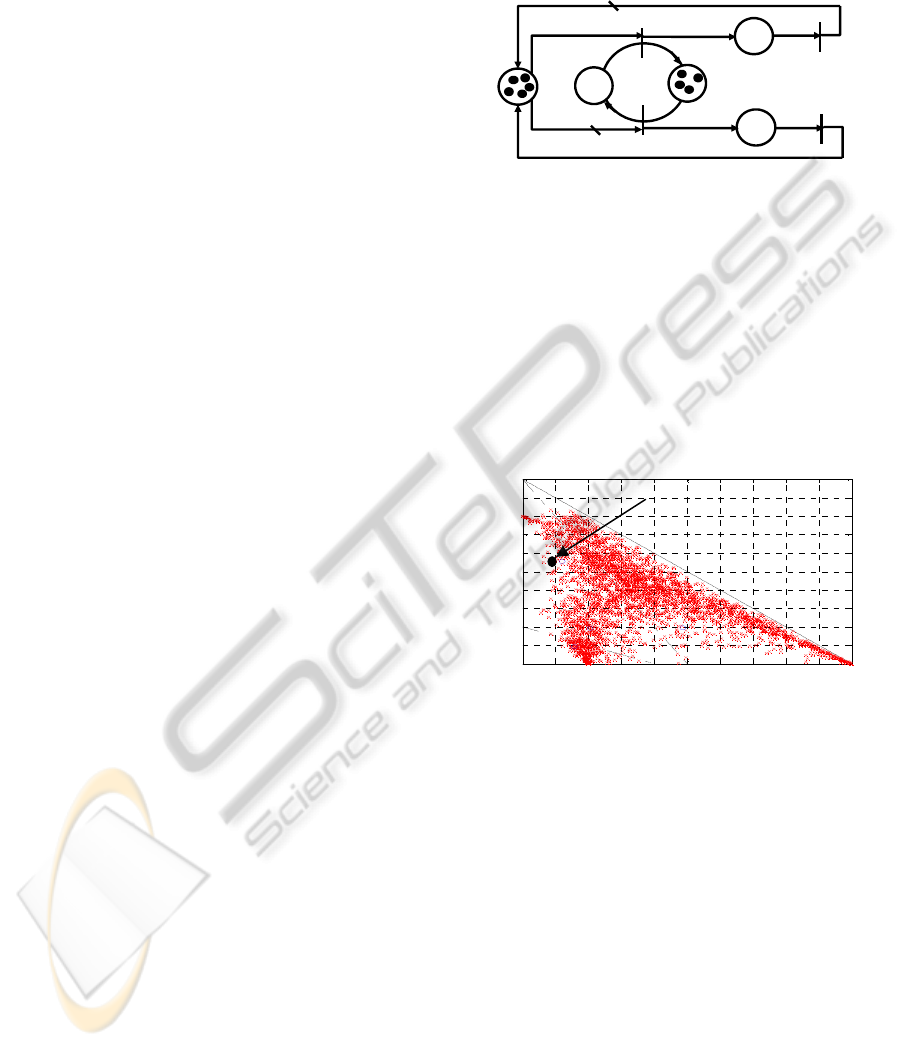
4 EXAMPLE
Consider for example the marked SPN described in
fig.1 (Julvez et al. 2005). This PN has 2 P-
semiflows: Y = ((0 0 0 1 1)
T
(1 1 2 1 0)
T
)
T
and C = (4
5)
T
. The subsets of places P
1
= {P
1
, P
2
, P
3
} and P
2
=
{P
4
, P5} are defined according to Y and lead to the
trivial transformation matrix D = I5 (i.e. M’ = M).
The fig. 2 illustrates stochastic mean markings that
are reached from MI = (5 0 0 0 4)T according to va-
rious transitions firing rate vectors [0 : 10]4.
Figure 1: An example of SPN with M
I
= (5 0 0 0 4)
T
.
If the PN of fig. 1 is considered as a CPN, 4 regions
A
1
to A
4
exist. The regions are defined by the
constraint matrices A
1
to A
4
.
1
1/20000
1 0000
0 1000
0 0100
A
2
1/20000
0 0010
01000
0 0100
A
3
00001
10000
01000
00100
A
4
00001
00010
01000
00100
A
The regions are also depicted in figures 2 to 4
according to the full lines (reachable area limits) and
dotted lines (regions intersections).
Figure 2: Projection in plan (m
1
, m
2
+ 2.m
3
) of M
mms
for
the SPN of fig. 1 with various vectors
[0 : 10]
4
.
The CPN as a single critical region A
1
and M
I
A
2
. The fig. 3 illustrates the asymptotic continuous
mean markings that are reached from M
I
and
according to various maximal firing speeds x
max j
[0.1 : 10], j = 1,…,4. Some areas in the critical
region A
1
are reachable with SPNs and not with
CPNs. For examples, the asymptotic mean markings
M
mms
(
) = (0.6 0.2 1.3 1.6 2.4)
T
obtained with
= (6
2 3 0.5)
T
is in critical region A
1
and is not reachable
with CPN (figs. 2 and 3): X
max
= diag(6 2 3 0.5)
T
leads to M
mmc
(X
max
) = (0.1 0.1 0.4 3.9 0.1)
T
and any
other maximal firing speeds also fail.
T
4
T
3
P
4
T
2
P
5
T
1
P
3
P
2
P
1
2
2
0 0.5 1 1.5 2 2.5 3 3.5 4 4.5 5
0
0.5
1
1.5
2
2.5
3
3.5
4
4.5
5
m
1
m
2
+2xm
3
M
mms
(
)
A
2
A
1
A
3
ICINCO 2010 - 7th International Conference on Informatics in Control, Automation and Robotics
366
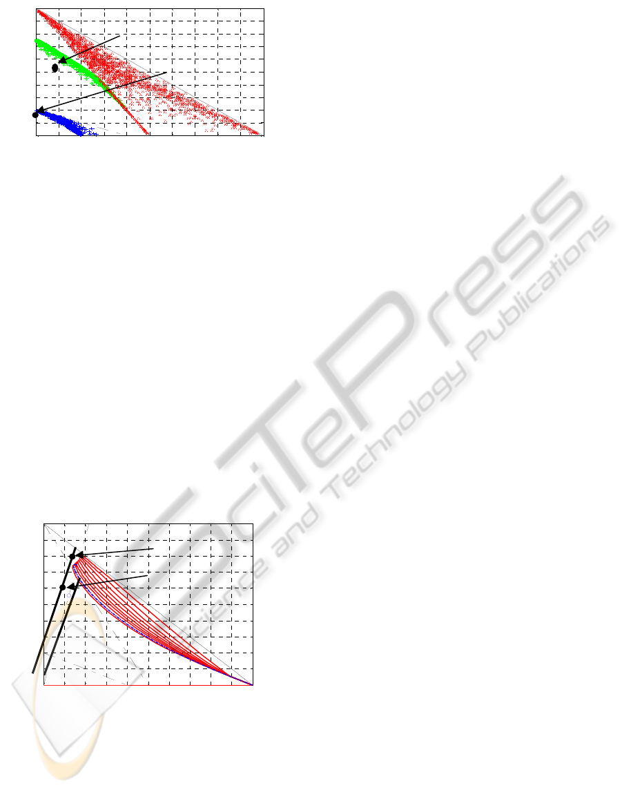
Figure 3: Projection in plan (m
1
, m
2
+2.m
3
) of M
mmc
for the
CPN of fig. 1 with various x
max j
[0.1 : 10], j=1,…,4.
The propositions 2 and 3 are used to work out the
admissible ratio
and the maximal firing speeds
that lead to homothetic approximations of
M
mms1
(SPN) . In the region A
2
, (7) leads to (10):
51
1
5
2
3
4
5
0
.'
0
.'
10010 0
..'
1/2000 1 4
"
5
"
4
5
x
mms
mms
mms
T
mms
T
mms
m
I
m
m
m
Y
m
Y
(9)
and then to the admissible interval
[5/(2.m
mms1
+
m
mms2
+2.m
mms3
) : 5/(m
mms1
+m
mms2
+2.m
mms3
)]. For the
considered example
[1.26: 1.48]. The figure 4
illustrates various homothetic marking trajectories
for SPN obtained for some values of parameter
in
admissible interval in order to reach
.M’
mms1
(μ).
Figure 4: Projection in plan (m
1
, m
2
+2.m
3
) of the
homothetic convergence to
.M’
mms
(μ).
The proposition 3 is used to work out the set of the
admissible maximal firing speeds that depend on the
parameter
such that the CPN with same structure
and initial marking tends to M
mms
:
x
max1
= 2.x
max4
.m
mms3
/ m
mms1
x
max2
=
.x
max4
. m
mms3
/ (5-
.(m
mms1
+m
mms2
+2.m
mms3
))
x
max3
= x
max4
m
mms3
/ m
mms2
(10)
where x
max4
is a dof. For example, consider the
particular homothetic ratio
= 4/3. The trajectory
(dotted line in figure 4), obtained for X
max
=(4.25,
3.41, 6, 1) results in asymptotic marking m’
mmc1
=
0.80, m’
mmc2
= 0.28, m’
mmc3
= 1.71. From this
approximation, it is easy to recover the asymptotic
stochastic mean marking M
mms
(
).
5 CONCLUSIONS
This paper has proposed partial homothetic
transformations of the SPN mean marking to
approximate. The proposed results concern the
existence of solutions but are not constructive in the
sense that the asymptotic stochastic mean markings
to estimate by CPNs must a priori be known. The
selection of the best projectors and ratios will be
investigated in our further works. Our future work is
also to investigate continuous approximations
directly derived from the SPNs transition firing
rates.
REFERENCES
Bobbio A., Puliafito A., Telek M., Trivedi K. (1998)
Recent Developments in Stochastic Petri Nets, J. of
Cir., Syst., and Comp., Vol. 8, No. 1, pp. 119--158.
David R., Alla H., (1992) Petri nets and grafcet – tools for
modelling DES, Prentice Hall, London.
Júlvez G., Recalde L. Silva M. (2005) Steady-state
performance evaluation of continuous mono-T-
semiflow Petri nets, Automatica, 41 (4), pp. 605-616.
Lefebvre D., Leclercq E., Khalij L., Souza de Cursi E., El
Akchioui N. (2009), Approximation of MTS
stochastic Petri nets steady state by means of
continuous Petri nets: a numerical approach, Proc.
IFAC ADHS, pp. 62-67, Zaragoza, Spain.
Lefebvre D., Leclercq E., (2010), Approximation of
Stochastic Petri Nets steady state by CPNs with
constant and piecewise-constant maximal firing
speeds, MOSIM 2010, Hammamet, Tunisia.
Molloy M.K., (1982) Performance analysis using
stochastic Petri nets, IEEE Tran. on Computers C, vol.
31, pp. 913 – 917.
Rausand M. and Hoyland A. (2004), System reliability
theory: models, statistical methods, and applications,
Wiley, Hoboken, New Jersey.
Silva M. and Recalde L. (2004) On fluidification of Petri
Nets: from discrete to hybrid and continuous models,
An. Reviews in Control, Vol. 28, no. 2, pp. 253-266.
Vazquez R., Recalde L., Silva M., (2008) Stochastic
continuous-state approximation of markovian Petri net
systems, Proc. IEEE – CDC08, pp. 901 – 906, Cancun,
Mexico.
0 0.5 1 1.5 2 2.5 3 3.5 4 4.5 5
0
0.5
1
1.5
2
2.5
3
3.5
4
4.5
5
a)
m
1
m
2
+ 2m
3
0 0.5 1 1.5 2 2.5 3 3.5 4 4.5 5
0
0.5
1
1.5
2
2.5
3
3.5
4
4.5
5
m1
m2+2m3
a
)
2
= 1.26
2
= 1.48
M
mms
(
)
.M’
mms1
(
)
M
mmc
(X
max
)
M
mms
(
)
A
2
A
1
A
3
HOMOTHETIC APPROXIMATIONS FOR STOCHASTIC PN
367
