ROBUST 6D POSE DETERMINATION IN COMPLEX

ENVIRONMENTS FOR ONE HUNDRED CLASSES

Thilo Grundmann, Robert Eidenberger, Martin Schneider and Michael Fiegert

Siemens AG, Corporate Technology, Autonomous Systems, Munich, Germany

Keywords:

Object recognition, 6d Pose estimation, Multi-object scenarios, SIFT, Large database, One-hundred classes.

Abstract:

For many robotic applications including service robotics robust object classiﬁcation and 6d object pose de-

termination are of substantial importance. This paper presents an object recognition methodology which is

capable of complex multi-object scenes. It handles partial occlusions and deals with large sets of different and

alike objects.

The object recognition process uses local interest points from the SIFT algorithm as features for object clas-

siﬁcation. From stereo images spatial information is gained and 6d poses are calculated. All reference data

is extracted in an off-line model generation process from large training data sets of a total of 100 different

household items. In the recognition phase these objects are robustly identiﬁed in sensor measurements.

The proposed work is integrated into an autonomous service robot. In various experiments the recognition

quality is evaluated and the position accuracy is determined by comparison to ground truth data.

1 INTRODUCTION

Object recognition comprises the tasks of object class

identiﬁcation and pose determination. Although this

plays a major role in several scientiﬁc domains, many

current approaches to object recognition are limited in

their applicability due to inaccuracies in the pose de-

termination, the number of detectable objects or the

complexity of scenes. Object occlusions and the ap-

pearance of similar objects in the same image often

constitute problems to robust detection.

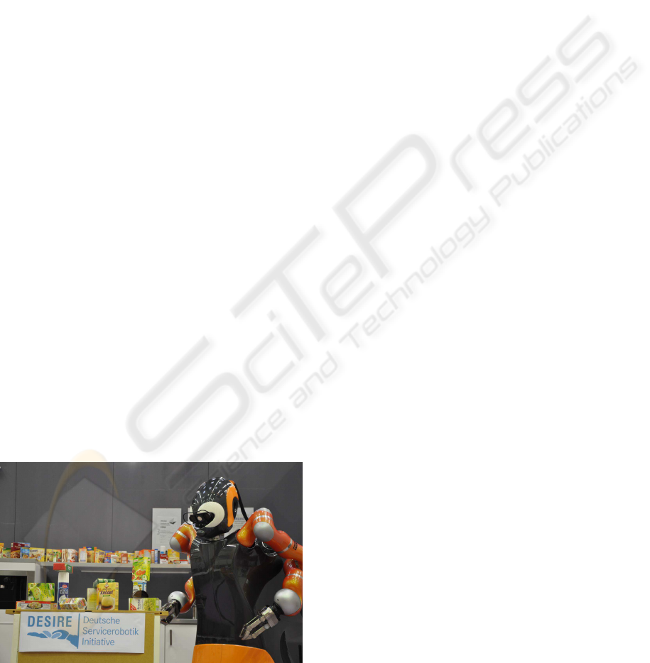
Figure 1: A service robot commonly operates in a complex

environment.

In this work we present a detection methodology

which allows accurate 6d object pose determination

and object class detection. It uses Lowe’s SIFT al-

gorithm (Lowe, 1999) for determining local, scale-

invariant features in images. The application of the

SIFT algorithm on stereo images from a camera pair

enables the calculation of precise object poses. This

appearance- and model-based approach consists of

two separate stages, Model generation and Object

recognition and pose determination.

Model generation is an off-line process, where the

object database is established by determining essen-

tial information from training data. We consider a set

of 100 household items of different or alike appear-

ance. The challenges lie in the reasonable acquisition

and efﬁcient processing and storing of large data sets.

Object recognition and pose determination aims

on satisfactory object classiﬁcation results, low mis-

classiﬁcation rates and fast processing. The precise

detection of the object pose allows the accurate po-

sitional representation of objects in a common refer-

ence frame which is important to many tasks. The 6d

pose is described by 3 translational and 3 rotational

components and is formulated in continuousdomains.

The proposed method is embedded in a mobile

service robotics framework. Figure 1 shows theproto-

type. The robust and accurate object recognition sys-

tem is basis to continuing works such as object mani-

301

Grundmann T., Eidenberger R., Schneider M. and Fiegert M. (2010).

ROBUST 6D POSE DETERMINATION IN COMPLEX ENVIRONMENTS FOR ONE HUNDRED CLASSES.

In Proceedings of the 7th International Conference on Informatics in Control, Automation and Robotics, pages 301-308

DOI: 10.5220/0002951403010308

 SciTePress

pulation (Xue et al., 2007), perception planning (Ei-

denberger et al., 2009) and physical object depen-

dency analysis (Grundmann et al., 2008), which point

out its importance.

Section 2 outlines current state of the art ap-

proaches to model generation and model-based object

recognition.

In Section 3 the data acquisition procedure and the

methodology for model generation is described. Sec-

tion 4 depicts the principles for object class identiﬁ-

cation and 6d pose determination.

This paper closes with experiments in Section 5

which demonstrate the proposed theoretical concepts

on real data.

2 RELATED WORK

The problemof visual object pose estimation has been

studied in the context of different ﬁelds of application,

robotics or augmented reality to name two.

All approaches can be characterized by a number

of parameters like the number of dimensions of the

measured pose (mostly one, three or six), the restric-

tions on the objects to be localized (e.g. in shape,

color or texture), the ability to estimate the pose of

multiple instances of the same class in one image and

the capacity for various different classes in the model

database of the proposed system. Also the proposed

sensor system (mono/stereo camera, resolution), pro-

cess runtime and the achieved precision in the pose

are characteristic.

One of the earlier papers on object pose estimation

(Nayar et al., 1996) dealt already with the high num-

ber of one hundred different classes. Nevertheless the

measured pose in this case is only one-dimensional,

and the scene is assumed to have a black background

and no occlusion or objects of unknown classes in it.

Later on (Zhang et al., 1999) and (Walter and Arn-

rich, 2000) extended the estimated pose to 3DOF as-

suming the objects to be located upright on a table,

using one of ﬁve objects in their experiments.

Others (Kragic et al., 2001) restricted their ob-

jects to forms that can be modeled by wire frames

and achieved good results in full 6d pose estimation

examining two different objects. The quality of the

pose is indirectly evaluated by successful grasping.

True 6d pose measurement using local SIFT fea-

tures was demonstrated by (Lowe, 1999), describing

a method that is able to localize ﬂat objects within

a range of 20 degrees, demonstrated on two scenes,

consisting of three different objects each, without

evaluation of the pose accuracy.

Azad et. al. presented a stereo camera based me-

thod (Azad et al., 2007) for full 6 DOF pose retrieval

of textured object using classic SIFT interest points.

The method requires the objects to posses ﬂat sur-

faces for the stereo recognition, and the accuracy of

the pose estimation is not measured directly.

Recently Collet et al. presented a mono camera

object localization system (Collet et al., 2009), based

on SIFT features using ransac and mean shift clus-

tering. They also describe an almost fully automatic

process for the model generation and give some ex-

periments with four object classes where measured

poses are evaluated against ground truth. The error

is described by histograms over the translational and

rotational error.

Another model generation system is described in

(Pan et al., 2009) which is able to build a model online

from a video stream. The model is also built fully

automatically, additionally the user is assisted in the

image collection by guiding the direction to which the

object should be moved and by the visual feedback of

the emerging model.

A comprehensive taxonomic and quantitative

comparison of multi-view stereo model building

methods for dense models can be found in (Seitz et al.,

2006), sparse models are out of scope for this paper

though.

Our approach is comparable to the method of

(Collet et al., 2009), using a similar 3d model which

is not restricted in the shape based on SIFT features.

Through the use of stereo vision and thus conceptual

different methods for the pose determination a higher

accuracy in pose measurement is achieved.

Note, that an exact direct comparison is difﬁcult

without perfect re-implementation, so we generated

translational and rotational histograms similar to the

ones in (Collet et al., 2009) which demonstrate a bet-

ter performance of our approach. But when it comes

to comparison, the main drawback to the research

done on six dimensional object localization is the ab-

sence of benchmark datasets.

3 MODEL GENERATION

Model generation aims on the acquisition of training

data and its processing to generate object class mod-

els. It is essential to ﬁlter signiﬁcant data and efﬁ-

ciently store it to enable reasonable processing times.

The KIT object modeling center IOMOS (Xue

et al., 2009) is shown in Figure 2 with its rotary

disk and the rotating bracket, where the sensors are

mounted on. A stereo camera system and a laser scan-

ner are used to acquire 360 stereo images for each

object and the 3d surface. Rotating the object on the

ICINCO 2010 - 7th International Conference on Informatics in Control, Automation and Robotics

302

Figure 2: Object modeling center.

turntable and moving the sensors results in sensor data

at 360

◦

latitudinal and 90

◦

longitudinal angles in 10

◦

steps.

The build process starts with computing the SIFT

interest points (IPs) for each image and calculates 3d

points by triangulation of IPs in each stereo image.

Then matches over all images are determined and

equivalence classes from these matching IPs found.

At last each equivalence class is represented by one

descriptor and one 3d location. All these equivalence

class representatives together build up the model.

Now, each step of the build process is described in

detail.

1. SIFT Interest Points Calculation. The base for

the process are the SIFT interest points for each im-

age. Each SIFT interest point s

= (u, v, s, o, d

) con-

sists of the 2d location (u, v) in the image, its scale

s and its orientation o. d

denotes the l-dimensional

descriptor vector. For each training image the set

of interest points in the left camera image S

with

= {s

, ...s

} is determined. The interest point set

for the right camera image is acquired respectively.

2. Triangulation. 3d points are computed for cor-

responding IP’s in the left and right images. Corre-

sponding IP’s are determined by using the epipolar

constraint and SIFT descriptor matching. For every

IP in a left image V

we compute the epipolar line

in the right image V

and determine the subset

⊂ {s

∈ S

|dist(s

, L

) < ε

} with ε

as the maxi-

mum epipolar distance. Then, SIFT descriptor match-

ing is performed. It is important to do the epipolar ex-

amination before the SIFT matching step. This way

the set of possible matches is constrained to a region

in the image. IPs with similar descriptors from other

parts are not considered and cannot distort the result.

For each matched IP pair (s

, s

) the corresponding 3d

location and orientation are computed using triangu-

lation (Hartley and Zisserman, 2004) and transformed

into the objects coordinate system to get the spatial

feature representation:

= (x, y, z, x

′

, y

′

, z

′

, s, o, d

). (1)

The ﬁrst three elements x,y and z denote the transla-

tional coordinates, x

′

and z

′

represent the direction

from where the interest point is visible. Scale s, orien-

tation o and descriptor d

are equal to the parameters

of the 2d interest point.

3. Equivalence Relation. The next step aims at par-

titioning this set of 3d points into subsets originating

from the same physical point. This equivalence re-

lation is seeded from IPs with ﬁtting appearance and

location and is completed by the transitive closure.

First candidates are found by appearance. The

enormous amount of data with on average 850 3d lo-

cations for each training view, 280000 for each object,

can be handled efﬁciently by means of a kd-tree. Us-

ing Euclidean distance in the SIFT descriptor space

the nearest n

- neighbors in the kd-tree are searched

for each s

depends on the sampling rate of the training

data as SIFT descriptors are only invariant within a

limited angular range and each face of the object is

only seen from a certain range of camera positions. It

was set to 150 in our case.

Then candidates are checked for their spacial ﬁt

by projecting them to the view of their matching part-

ner both ways and calculating the Euclidean distance

in the image. If this distance, which is the expected

reprojection error, exceeds a threshold (5 pixel in our

system) the candidate is rejected. In rare cases it can

happen that two IP’s from the same view are in one

equivalence class. These IP’s are removed.

A standard connected component algorithm is

used to compute the transitive closure.

4. Subdivision and Representatives. We now seek

a simple representation for each equivalence class

above a minimal size v

min

. Very small classes (eg.

min

=4) are discarded to suppress IPs of low value for

the recognition process and noise.

When evaluating classes one ﬁnds the locations

clustering well, but descriptors to spread consider-

ably. This is not surprising since we do see most

points from a wide angle range were the SIFT descrip-

tor cannot be assumed to be invariant. Instead of more

complex density models we favor a very simple rep-

resentative, which is a simple mean for location and

normalized mean for descriptor. To make this simple

model suitable we sacriﬁce the simple relation, where

one class corresponds to one physical point, and split

classes with k-means until they can be represented as

spheres. This considerably simpliﬁes and speeds up

the recognition process.

ROBUST 6D POSE DETERMINATION IN COMPLEX ENVIRONMENTS FOR ONE HUNDRED CLASSES

303

Figure 3: Sensor head: Stereo cameras and 3d-TOF camera

mounted on a pan/tilt unit.

The full model for one object needs about 5% of stor-

age of the initial SIFT features. This enables fast

recognition since big databases can be held in RAM

completely.

4 OBJECT RECOGNITION AND

POSE DETERMINATION

Many applications require a high pose determination

accuracy. To account for this we use a stereo cam-

era based approach, as preceding experiments using

a mono camera and the posit algorithm (Dementhon

and Davis, 1995) lead to unsatisfying results. Compa-

rable results were found in (Azad et al., 2009) which

showed that stereo approaches outperformmono cam-

era approaches by the factor of ≈ 2.

Our stereo setup on the robot (Figure3) consists of

two AVT Pike F-145C ﬁrewire cameras with a resolu-

tion of 1388 x 1038 pixels each, equippedwith 8.5mm

objectives and mounted with a disparity of 0.12m.

Precise intrinsic and stereo calibration of the cam-

eras is essential to our algorithms so they were carried

out with the Camera Calibration Toolbox for MAT-

LAB, using about 60 stereo image pairs of a custom

made highly planar checkers calibration pattern.

The recognition and localization process consists

of the following steps:

1. Calculate SIFT Interest Points. For each of the

stereo images, V

and V

a corresponding set of in-

terest points is calculated S

= {s

, ..., s

} and S

, ..., s

2. Find Correspondence to Object Models

(Figure4). For all elements s

∈ S

try to ﬁnd up to

multiple matches c

= {i, j} with a 3d feature

from the model database s

∈ M. The criterion for

a match is that the Euclidean distance in descriptor

space is below an absolute threshold p

= 0.3. The

multiple match is needed, because with an increasing

Figure 4: Recognition principle: ﬁnding matches between

interest points s

∈ M from given models and interest points

detected in one image s ∈ S

(step 2).

number of object models in the database, the unique-

ness of a lot of features is lost. This happens in a non

ignorable way for household items that often follow a

corporate design and share large areas of texture.

To speed up the search for matches, the descrip-

tors from the database M are structured in a kd-tree

using the ANN library. To increase the performance,

the nearest neighbor search is approximated. The

quality of the approximation can be parameterized,

we used the value p

app

= 5.

3. Construct Stereo Interest Points. For all match-

ings c

= {i, j}, we try to ﬁnd multi stereo matches on

the right interest point set S

. The epipolar constraint

is used in the same manner as described in Section

3.2, but after the epipolar spatial restriction, a relative

multi match is used. This has to be done to account for

the classic situation where multiple instances of the

same object class are placed side by side on a board,

leading to multiple similar features on the epipolar

line L

. After this procedure we obtain a set of l 3d

SIFT points S



, ..., s



by triangulation. Each

of these 3d SIFT points belongs to an object class, in-

dicated by its corresponding database feature s

. In

a system with t known classes this gives a partition

of S



, ..., S



, whereas some of these class de-

pending partitions might be empty. From here on, all

calculation is done separately for each object class.

4. Cluster within Class t. To account for scenes

with large numbers of identical objects and to deal

with the high number of erroneous 3d SIFT features,

we construct initial pose estimates P =



, ..., p



from S

. This is done by choosing randomly

non collinear triplets of 3d interest points from S

and check whether their mutual Euclidean distances

ICINCO 2010 - 7th International Conference on Informatics in Control, Automation and Robotics

304

match those in the model database.

Within the 6d space of the initial pose estimates P,

qt-clustering (Heyer et al., 1999) is performed to ﬁnd

consistent 6d pose estimates. The clusters consist of

6d poses p

which all correspond to a triplet of 3d

interest point S

. That way each cluster describes a

set of 3d interest points S

⊂ S

5. Pose Determination. All 3d interest points from

each cluster S

are used to determine the transforma-

tion of the database 3d IPs into the measured cloud

by a least squares pose ﬁt (Figure 4). In the resulting

list of object classes and poses a similarity search is

performedto eliminate duplicate poses, which emerge

from imperfect clustering.

One important advantage of this 3d SIFT stereo ap-

proach is, that in contrast to other approaches it is able

to handle objects of any shape, as long as the object

fulﬁlls the requirements on its texture that are inher-

ent to the SIFT algorithm. It is not generally bound to

the usage of SIFT features, so in the future improved

interest point methods could replace the SIFT inter-

est points. Note, that the parameters in the algorithm

strongly inﬂuence the performance and thus have to

be optimized to ﬁt an application scenario.

5 EXPERIMENTS

The experiments we conducted should evaluate the

performance of our system in terms of detection rate

and pose accuracy. Since it is very difﬁcult to acquire

pose ground truth data in complex scenarios we split

the evaluation into two parts. In the ﬁrst part, we set

up scenes where the ground truth pose can be deter-

mined with a calibration pattern, leading to single ob-

ject scenes of low complexity. The detection rate in

these simple settings was 100%.

In order to evaluate our method in more realistic

scenarios, we set up a second test, based on complex

scenes consisting of up to 30 objects placed in arbi-

trary positions in a real environment supplemented

with unknown objects. This way the method’s robust-

ness against occlusion, object ambiguities and envi-

ronmental inﬂuences can be evaluated. In such sce-

narios, ground truth poses are not available, but it is

possible to evaluate the correctness of the detection

by visual inspection of the bounding volumes that are

projected into the images.

The time required for a one shot recognition of a

complete scene can be divided up into two parts: The

SIFT calculation takes about 0.6 seconds per image

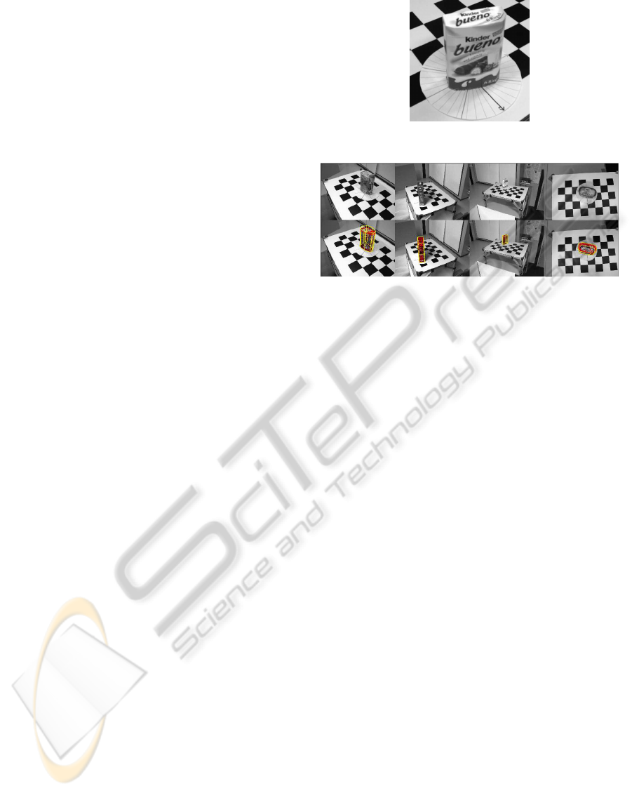
Figure 5: Object with calibration sheet.

Figure 6: 1st row: objects, placed precisely onto the cal-

ibration pattern. 2nd row: Ground truth values projected

into image (dot cloud(red), bounding volume(yellow)).

on a 2GHz Intel multicore and the processing of the

poses takes 0.3 seconds without using the multi cores.

Note that there are some parameters like the kd-tree

approximation quality which strongly inﬂuence the

runtime of the processing part.

5.1 Evaluation of Pose Accuracy

To evaluate the system’s accuracy in the pose esti-

mation, we compared the recognition results of 260

scenes with ground truth. To acquire 6d ground

truth data we applied paper sheets with the projected

corresponding model onto the bottom of the objects

(Figure5). Since the origin of the objects is located in

the bottom plane, this method enables us to place the

object onto a calibration pattern with 3DOF and with

sub-millimeter accuracy.

In the test we placed one object per scene onto a

calibration pattern (Figure6) and measured its pose.

Using the camera’s pose with reference to the cali-

bration pattern which is determined using the Mat-

lab calibration toolbox, we transformed the ground

truth pose into the camera coordinate frame where

we compared it against the result of the recognition

algorithm. We selected seven different objects with

varying shapes for this experiment.

The distance of the objects origin and the camera

ranged from 0.42m to 1.25m (Figure 7/1). This area

was chosen from our experiences with the working

area of the mobile service robot.

Due to the relatively simple nature of the scenes

all objects were detected correctly, so we collected

260 pose measurement error vectors. As expected

ROBUST 6D POSE DETERMINATION IN COMPLEX ENVIRONMENTS FOR ONE HUNDRED CLASSES

305

Figure 7: 1st: Histogram of object’s distance to camera over

the test set. 2nd: Translational error over distance (dots) and

the mean translational error over distance (bars).

Figure 8: Histograms of translational(in cm) and rotational

error(in ◦).

from the measurement principle, the results show in-

creasing translational errors with growing distance

(Figure7/2). For the evaluation of the rotational er-

rors, we calculated the minimal rotation angle from

the resulting 6d pose to the ground truth 6d pose. The

overall distribution of translational and rotational er-

rors are shown in Figure 8, the corresponding stan-

dard deviation of the translational error is shown in

Table 1.

To get a more expressive model of this mea-

surement process, we transformed the error into the

camera frame, and calculated the covariance for the

translational components of the measurement errors

(Figure9). As expected from the measurement princi-

ple, the standard deviation of the z

-component in the

camera frame is considerably higher as the standard

Figure 9: The xyz-deviations of all test scenes, depicted in

the camera frame, with its covariance ellipsoid (95% quan-

tile).

Table 1: Translational error in the camera frame.

stddev [mm]

k(x

2.2436

1.3763

1.3617

3.4235

deviations in the other directions x

and y

(Tab.1).

Using this model it is possible to model detection in-

accuracies fairly precisely. Note, that the inaccuracies

also contain potential errors in the 3d models as well

as the bias from placing the object imprecisely onto

calibration pattern.

5.2 Object Recognition in Complex

Environments

In this experiment complex and cluttered scenes are

considered. A series of 60 images of different scenar-

ios at different locations are investigated. All contain

chaotic object arrangements including trained and un-

known, random objects. For the evaluation, all ob-

jects are categorized according to their distance from

the camera and to their occlusions. Thus, we differen-

tiate between close and far items and cluster the ob-

jects into fully visible, partly occluded and heavily

occluded ones.

Figures 10(a) and 10(d) show two scenes with the

initially labeled objects. Squares mark fully visible

objects, diamonds indicate partly occluded items and

circles denote heavily occluded ones. Close objects

are shown solid, far away objects as halves. The yel-

low area on the left of these images is not considered

for the stereo matching, so objects in this part of the

image are ignored for the recognition. The respective

detection and classiﬁcation results for the two scenes

are illustrated in Figures 10(b) and 10(e). The bound-

ing volumes with respect to the 6d poses of the recog-

nized objects are projected into the image. In the ﬁrst

sample, all objects are detected. However, a small

number of false positives can be recognized for the

salt boxes, the rye bread and the oil can. False pos-

itives are objects that are detected although they are

not physically there. They result from ambiguous ob-

jects with similar textures on several sides or similar

objects in the database, such as the three almost iden-

tical salts. In Figure 10(e) not all objects are recog-

nized because of heavier occlusions. Though, fully

visible ones are clearly identiﬁed. The successful de-

tection also depends on the lighting as the trained im-

ages were acquired under one speciﬁc lighting condi-

tion. Variations inﬂuence the recognition process.

By visual inspection the detection results are com-

ICINCO 2010 - 7th International Conference on Informatics in Control, Automation and Robotics

306

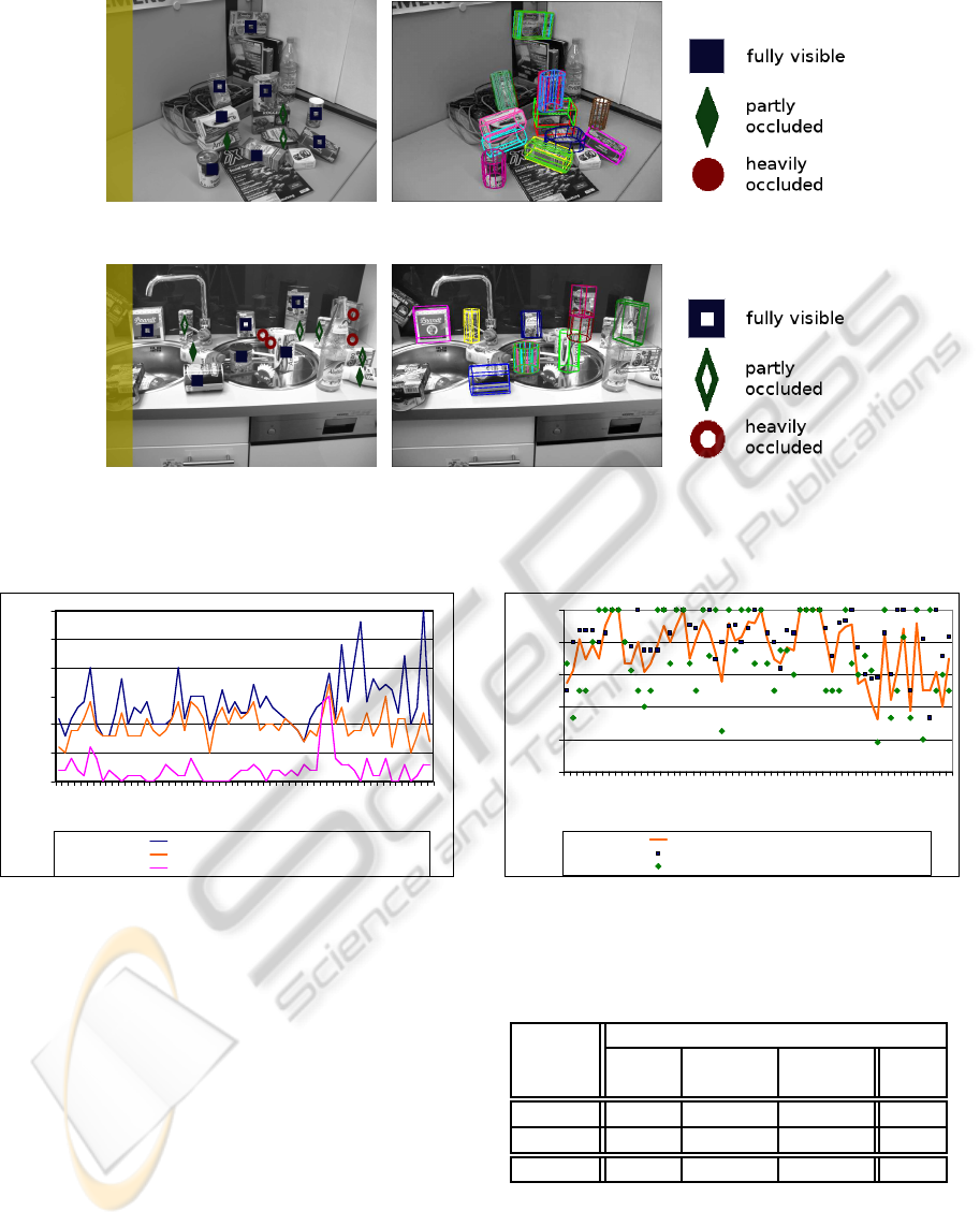
(a) Labeled ofﬁce scene (b) Detection results (c) Legend (near ob-

jects)

(d) Labeled kitchen scene (e) Detection results (f) Legend (far objects)

Figure 10: One shot detection results for two complex scenes in a kitchen and an ofﬁce environment. The results are evaluated

with respect to the a priori categorized objects.

1 5 9 13 17 21 25 29 33 37 41 45 49 53 57

Test series

Number of objects

Total number of objects

Number of detected objects

False positives

Figure 11: Object detection results and false positives in

comparison to the total number of objects in scene for 60

different scenarios with a total of 826 objects.

pared to the pre-selection. The true positive and false

positive classiﬁcations rates are manually determined

by checking the class and pose recognition results.

Figure 11 shows the detection results of each of the 60

scenarios. The total number of objects in the scenes

ranges from 7 to 30. The number of recognized ob-

jects and the false positives for each scene are also

plotted. While the number of false positives is gener-

ally low, a few scenes with very dense object arrange-

ments showed more than 10 false object hypotheses.

In Figure 12 the detection rates are plotted. The

overall rates show the number of detected objects over

the total objects in the scene. The other curves depict

the rate of detecting fully visible objects and partly

occluded ones. The total recognition results over all

0.2

0.4

0.6

0.8

1 4 7 10 13 16 19 22 25 28 31 34 37 40 43 46 49 52 55 58

Test series

Detection rate

Total detection rate

Fully visible detection rate

Partly occluded detection rate

Figure 12: Overall detection rate and detection rates of fully

visible and partially occluded objects.

Table 2: Object class detection results broken down to the

detection categories.

detection rates

fully partly heavily

distance visible occluded occluded total

near 0.863 0.763 0.179 0.796

far 0.813 0.593 0.167 0.617

total 0.846 0.684 0.170 0.722

scenes are listed in Table 2. Rates for each category

a separately and jointly determined. As expected,

closer objects perform better in the recognition. In

matters of occlusions, a decay can be recognized from

fully visible to heavily occluded items. The overall

detection rate of 72 per cent is lower than the peak

ROBUST 6D POSE DETERMINATION IN COMPLEX ENVIRONMENTS FOR ONE HUNDRED CLASSES

307

detection rate of 86 per cent for close and fully visi-

ble objects. The random object alignments with un-

favorable object poses, lighting inﬂuences and object

occlusions are reasons for recognition failures. How-

ever, considering the large database and the complex-

ity of the scenes the one shot recognition results are

promising.

6 CONCLUSIONS

We presented a system that is able to detect and lo-

calize objects from up to 100 different classes. The

6d detection accuracy of the object pose and the de-

tection rate are evaluated in extensive experiments,

which demonstrated a true positive detection rate of

72% in highly complex cluttered multi object scenes

with partly occlusions. The resulting pose errors had

a standard deviation of 3.4mm in the direction of the

camera (z

) and 1.4mm in x

and y

A satisfactory trade-off is found between fast pro-

cessing and good recognition rates and detection er-

rors and failure recognitions. The system is suitable

to applications in cluttered environments with random

object alignments and unknown objects.

In future works, we plan to include sparse bun-

dle adjustment into the model generation process to

increase the precision in the 3d models which is ex-

pected to increase the pose precision on the one hand,

but also to loosen the precision requirements on the

camera pose.

ACKNOWLEDGEMENTS

This work has partly been supported by the German

Federal Ministry of Education and Research (BMBF)

under grant no. 01IME01D, DESIRE.

REFERENCES

Azad, P., Asfour, T., and Dillmann, R. (2007). Stereo-

based 6d object localization for grasping with hu-

manoid robot systems. In IEEE IROS 2007.

Azad, P., Asfour, T., and Dillmann, R. (2009). Stereo-based

vs. monocular 6-dof pose estimation using point fea-

tures: A quantitative comparison. In Autonome Mo-

bile Systeme 2009, Informatik aktuell. Springer.

Collet, A., Berenson, D., Srinivasa, S., and Ferguson, D.

(2009). Object recognition and full pose registration

from a single image for robotic manipulation. In IEEE

ICRA 09.

Dementhon, D. F. and Davis, L. S. (1995). Model-based ob-

ject pose in 25 lines of code. International Journal of

Computer Vision, Springer Netherlands, Volume 15.

Eidenberger, R., Grundmann, T., and Zoellner, R. (2009).

Probabilistic action planning for active scene model-

ing in continuous high-dimensional domains. IEEE

ICRA 2009.

Grundmann, T., Eidenberger, R., and Zoellner, R. (2008).

Local dependency analysis in probabilistic scene esti-

mation. In ISMA 2008. 5th International Symposium

on Mechatronics and Its Applications.

Hartley, R. and Zisserman, A. (2004). Multiple View Geom-

etry in Computer Vision. Cambridge University Press.

Heyer, L. J., Kruglyak, S., and Yooseph, S. (1999). Ex-

ploring expression data: Identiﬁcation and analysis of

coexpressed genes. Genome Res., 9.

Kragic, D., Miller, A. T., and Allen, P. K. (2001). Real-time

tracking meets online grasp planning. In IEEE ICRA

2001, Seoul, Republic of Korea.

Lowe, D. G. (1999). Object recognition from local scale-

invariant features. In International Conference on

Computer Vision, pages 1150–1157, Corfu, Greece.

Nayar, S., Nene, S., and Murase, H. (1996). Real-time 100

object recognition system. In IEEE ICRA 1996.

Pan, Q., Reitmayr, G., and Drummond, T. (2009). Pro-

FORMA: Probabilistic Feature-based On-line Rapid

Model Acquisition. In Proc. 20th British Machine Vi-

sion Conference (BMVC), London.

Seitz, S. M., Curless, B., Diebel, J., Scharstein, D., and

Szeliski, R. (2006). A comparison and evaluation of

multi-view stereo reconstruction algorithms. In IEEE

CVPR 2006.

Walter, J. A. and Arnrich, B. (2000). Gabor ﬁlters for object

localization and robot grasping. In ICPR 2000.

Xue, Z., Kasper, A., Zoellner, J., and Dillmann, R.

(2009). An automatic grasp planning system for ser-

vice robots. In 14th International Conference on Ad-

vanced Robotics (ICAR).

Xue, Z., Marius Zoellner, J., and Dillmann, R. (2007).

Grasp planning: Find the contact points. In IEEE Ro-

bio 2007.

Zhang, J., Schmidt, R., and Knoll, A. (1999). Appearance-

based visual learning in a neuro-fuzzy model for ﬁne-

positioning of manipulators. In IEEE ICRA 1999.

ICINCO 2010 - 7th International Conference on Informatics in Control, Automation and Robotics

308